6 Alternative approaches to population synthesis
This chapter briefly describes other techniques for spatial microsimulation. We have different methods, each corresponding to a section:
- GREGWT (6.1) contains a method based on a Generalized Regression Weighting procedure.
- Population synthesis as an optimization problem (6.2) explains how we can make spatial microsimulation thanks to optimization algorithms.
- simPop (6.3) mentions another package to make spatial microsimulation.
- The Urban Data Science Toolkit (UDST) (6.4) shortly describes another technique, coded in python.
6.1 GREGWT
As described in the Introduction, IPF is just one strategy for obtaining a spatial microdataset. However, researchers tend to select one method that they are comfortable with and stick with that for their models. This is understandable because setting up the method is usually time consuming: most researchers rightly focus on applying the methods to the real world rather than fretting about the details. On the other hand, if alternative methods work better for a particular application, resistance to change can result in poor model fit. In the case of very large datasets, spatial microsimulation may not be possible unless certain methods, optimised to deal with large datasets, are used. Above all, there is no consensus about which methods are ‘best’ for different applications, so it is worth experimenting to identify which method is most suitable for each application.
An interesting alternative to IPF method is the GREGWT algorithm. First implemented in the SAS language by the Statistical Service area of the Australian Bureau of Statistics (ABS), the algorithm reweighs a set of initial weights using a Generalized Regression Weighting procedure (hence the name GREGWT). The resulting weights ensure that, when aggregated, the individuals selected for each small area fit the constraint variables. Like IPF, the GREGWT results in non-integer weights, meaning some kind of integerisation algorithm will be needed to obtain individual level microdata. For example, if the output is to be used in ABM, the macro developed by ABS adds a weight restriction in their GREGWT macros to ensure positive weights. The ABS uses the Linear Truncated Method described in Singh and Mohl (1996) to enforce these restrictions.
A simplified version of this algorithm (and other algorithms) is provided by Rahman (2009). The algorithm is described in more detail in Tanton et al. (2011). An R implementation of GREGWT can be found in the GitHub repository GREGWT and installed using the function install_github() from the devtools package.
The code below uses this implementation of the GREGWT algorithm, with the data from Chapter 3.
# Install GREGWT (uncomment/alter as appropriate)
# devtools::install_github("emunozh/GREGWT")
# load the library (0.7.3)
library('GREGWT')

# Load the data from csv files stored under data
age = read.csv("data/SimpleWorld/age.csv")
sex = read.csv("data/SimpleWorld/sex.csv")
ind = read.csv("data/SimpleWorld/ind-full.csv")
# Make categories for age
ind$age <- cut(ind$age, breaks=c(0, 49, Inf),
               labels = c("a0.49", "a.50."))
# Add initial weights to survey
ind$w <- vector(mode = "numeric", length=dim(ind)[1]) + 1

# prepare simulation data using GREGWT::prepareData
data_in <- prepareData(cbind(age, sex),
                  ind, census_area_id = F, breaks = c(2))

# prepare a data.frame to store the result
fweights <- NULL
Result <- as.data.frame(matrix(NA, ncol=3, nrow=dim(age)[1]))
names(Result) <- c("area", "income", "cap.income")
The code presented above loads the SimpleWorld data and creates a new data.frame with this data. Version 1.4 of the R library requires the data to be in binary form. The require input for the R function is X representing the individual level survey, dx representing the initial weights of the survey and Tx representing the small area benchmarks.
# Warning: test code
# loop through simlaton areas
for(area in seq(dim(age)[1])){
    gregwt = GREGWT(data_in = data_in, area_code = area)
    fw <- gregwt$final_weights
    fweights <- c(fweights, fw)
    ## Estimate income
    sum.income <- sum(fw * ind$income)
    cap.income <- sum(fw * ind$income / sum(fw))
    Result[area,] <- c(area, sum.income, cap.income)
}
In the last step we transform the vector into a matrix and see the results from the reweighing process.
6.2 Population synthesis as an optimization problem
In general terms, an optimization problem consists of a function, the result of which must be minimised or maximised, called an objective function. This function is not necessarily defined for the entire domain of possible inputs. The domain where this function is defined is called the solution space (or the feasible space in formal mathematics). Moreover, optimization problems can be unconstrained or constrained, by limits on the values that arguments (or that a function of the arguments) of the function can take (Boyd 2004). If there are constraints, the solution space could include only a part of the image of the objective function. The objective function and the constraints are both necessary to define the solution space. Under this framework, population synthesis can be seen as a constrained optimisation problem. Suppose \(x\) is a vector of length \(n\) \((x_1,x_2,..,x_n)\) whose values are to be adjusted. In this case the value of the objective function is \(f_0(x)\), depends on \(x\). The possible values of \(x\) are defined thanks to par, a vector of predefined arguments or parameters of length \(m\) (\(m\) is the number of constraints) (\(par_1,par_2,..,par_m\)). This kind of problem can be expressed as:
\[\left\{ \begin{array}{l} min \hspace{0.2cm}f_0(x_1,x_2,..,x_n) \\ \\ s.c. \hspace{0.2cm} f_i(x) \geq par_i,\ i = 1, ..., m \end{array} \right.\]
Applying this to the problem of population synthesis, the parameters \(par_i\) represent 0 and \(f_i(x)=x\), since all cells have to be positive. The \(f_0(x)\) to be minimised is the distance between the actual weight matrix and the aggregate constraint variable cons. \(x\) represents the weights which will be calculated to minimise \(f_0(x)\).
To illustrate the concept further, consider the case of aircraft design. Imagine that the aim (the objective function) is to minimise weight by changing its shape and materials. But these modifications must proceed subject to some constraints, because the airplane must be safe and sufficiently voluminous to transport people. Constrained optimisation in this case would involve searching combinations of shape and material (to include in \(x\)) that minimise the weight (the result of \(f_0\), is a single value depending on \(x\)). This search must take place under constraints relating to volume (depending on the shape) and safety (\(par_1\) and \(par_2\) in the above notation). Thus \(par\) values define the domain of the solution space. We search inside this domain for the combination of \(x_i\) that minimises weight.
The case of spatial microsimulation has relatively simple constraints: all weights must be positive or zero:
\[ \left\{ weight_{ij} \in \mathbb{R}^+ \cup \{0\} \hspace{0.5cm} \forall i,j \right\} \]
Seeing spatial microsimulation as an optimisation problem allows solutions to be found using established techniques of constrained optimisation. The main advantage of this reframing is that it allows any optimisation algorithm to perform the reweighting.
To see population synthesis as a constrained optimization problem analogous to aircraft design, we must define the problem to optimise the variable \(x\) and then set the constraints.
Intuitively, the weight (or number of occurrences) for each individual should be the one that best fits the constraints. We could take the weight matrix as \(x\) and as the objective function the difference between the population with this weight matrix and the constraint. However, we want to include the information of the distribution of the sample. We must find a vector w with which to multiply the indu matrix. indu is similar to ind_cat, but each row of ind_cat represents an individual of the sample, whereas each row of indu concerns a type of individual. This means that if 2 people in the sample have the same characteristics, the corresponding line in indu will appear only once. The cells of indu contain the number of times that this kind of individual appears in the sample. The result of this multiplication should be as close as possible to the constraints.
When running the IPF procedure zone-by-zone using this method, the optimization problem for the first zone can be written as follows:
\[\left\{ \begin{array}{l} min \hspace{0.2cm} f(w_1,..,w_m) = DIST(sim, cons[1,]) \\ \hspace{0.8cm} where \hspace{0.2cm} sim=colSums(indu * w)\\ \\ s.c. \hspace{0.2cm} w_i \geq 0,\ i = 1, ..., m \end{array} \right.\]
Key to this is interpreting individual weights as parameters (the vector \(w=(w_1,...,w_m)\), of length \(m\) above) that are iteratively modified to optimise the fit between individual and aggregate level data. Note that in comparison with the theoretical definition of an optimisation problem, our parameters to determine (par) are the theoretical \(x\). The measure of fit, so the distance, we use in this context is Total Absolute Error (TAE).
\[\left\{ \begin{array}{l} min \hspace{0.2cm} f(w_1,..,w_m) = TAE(sim, cons[1,]) \\ \hspace{0.8cm} where \hspace{0.2cm} sim=colSums(ind\_cat * w)\\ \\ s.c. \hspace{0.2cm} w_i \geq 0,\ i = 1, ..., m \end{array} \right.\]
Note that although the “TAE” goodness-of-fit measure was used in this example, any could be used.
Note that in the above, \(w\) is equivalent to the weights object we have created in previous sections to represent how representative each individual is of each zone.
The main issue with this definition of reweighting is therefore the large number of free parameters: equal to the number of individual level dataset. Clearly this can be very very large. To overcome this issue, we must ‘compress’ the individual level dataset to its essence, to contain only unique individuals with respect to the constraint variables (constraint-unique individuals).
The challenge is to convert the binary ‘model matrix’ form of the individual level data (ind_cat in the previous examples) into a new matrix (indu) that has fewer rows of data. Information about the frequency of each constraint-unique individual is kept by increasing the value of the ‘1’ entries for each column for the replicated individuals by the number of other individuals who share the same combination of attributes. This may sound quite simple, so let’s use the example of SimpleWorld to illustrate the point.
6.2.1 Reweighting with optim and GenSA
The base R function optim provides a general purpose optimization framework for numerically solving objective functions. Based on the objective function for spatial microsimulation described above, we can use any general optimization algorithm for reweighting the individual level dataset. But which to use?
Different reweighting strategies are suitable in different contexts and there is no clear winner for every occasion. However, testing a range of strategy makes it clear that certain algorithms are more efficient than others for spatial microsimulation. Figure 6.1 demonstrates this variability by plotting total absolute error as a function of number of iterations for various optimization algorithms available from the base function optim and the GenSA package. Note that the comparisons are performed only for zone 1.
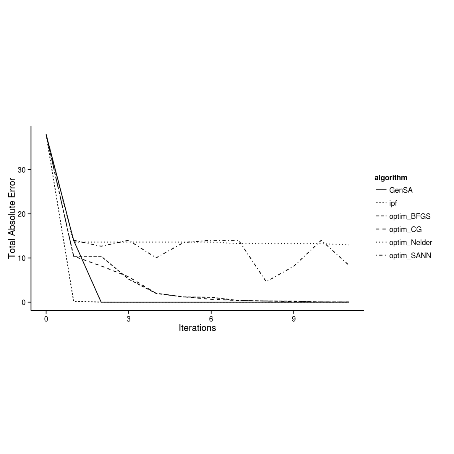
Figure 6.1: Relationship between number of iterations and goodness-of-fit between observed and simulated results for different optimisation algorithms.
Figure 6.1 shows that all algorithms improve fit during the first iteration. The reason for using IPF becomes clear after only one iteration. On the other end of the spectrum is R’s default optimization algorithm, the Nelder-Mead method, which requires many more iterations to converge to a value approximating zero than does IPF.22 Next best in terms of iterations is GenSA, the Generalized Simulated Annealing Function from the GenSA package. GenSA attained a near-perfect fit after only two full iterations.
The remaining algorithms shown are, like Nelder-Mead, available from within R’s default optimisation function optim. The implementations with method = set to "BFGS" (short for the Broyden–Fletcher–Goldfarb–Shanno algorithm), "CG" (‘conjugate gradients’) performed roughly the same, steadily approaching zero error and fitting to "IPF" and "GenSA" after 10 iterations. Finally, the SANN method (a variant of a Simulated ANNealing), also available in optim, performed most erratically of the methods tested. This is another implementation of simulated annealing which demonstrates that optimisation functions that depend on random numbers do not always lead to improved fit from one iteration to the next. If we look until 200 iterations, the fit will continue to oscillate and not be improved at all.
The code used to test these alternative methods for reweighting are provided in the script ‘code/optim-tests-SimpleWorld.R’. The results should be reproducible on any computer, provided the book’s supplementary materials have been downloaded. There are many other optimisation algorithms available in R through a wide range of packages and new and improved functions are being made available all the time. Enthusiastic readers are encouraged to experiment with the methods presented here: it is possible that an algorithm exists which outperforms all of those tested for this book. Also, it should be noted that the algorithms were tested on the extremely simple and rather contrived example dataset of SimpleWorld. Some algorithms may perform better with larger datasets than others and may be sensitive to changes to the initial conditions such as the problem of ‘empty cells’.
Therefore these results, as with any modelling exercise, should be interpreted with a healthy dose of skepticism: just because an algorithm converges after few ‘iterations’ this does not mean it is inherently faster or more useful than another. The results are context specific, so it is recommended that the tested framework in ‘code/optim-tests-SimpleWorld.R’ is used as a basis for further tests on algorithm performance on the datasets you are using. IPF has performed well in the situations I have tested it in (especially via the ipfp function, which performs disproportionately faster than the pure R implementation on large datasets) but this does not mean that it is always the best approach.
To overcome the caveat that the meaning of an ‘iteration’ changes dramatically from one algorithm to the next, further tests measured the time taken for each reweighting algorithm to run. To have a readable graph, we do not represent the error as a function of the time, but the time per algorithm in function of the number of iterations (Figure 6.2). This figure demonstrates that an iteration of GenSA take a long time in comparison with the other algorithm. Moreover, "BFGS" and "CG" are still following a similar curve under GenSA. Nelder-Mead, SANN and IPF contains iterations that take less time. By observing Figures 6.1 and 6.2 simultaneously , it appears that IPF is the best in terms of convergence (little TAE after few iterations) and the time needed for few iterations is good.
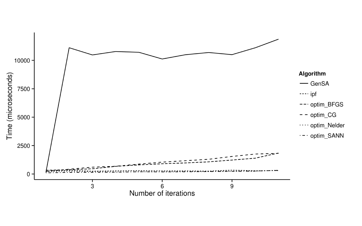
Figure 6.2: Relationship between processing time and goodness-of-fit between observed and simulated results for different optimisation algorithms.
Nelder-Mead is fast at reaching a good approximation of the constraint data, despite taking many iterations. GenSA, on the other hand, is shown to be much slower than the others, despite only requiring 2 iterations to arrive at a good level of fit.
Note that these results are biased by the example that is pretty small and runs only for the first zone.
6.2.2 Combinatorial optimisation
Combinatorial optimisation (CO) is a set of methods for solving optimisation problems from a discrete range of options. Instead of allocating weights to individuals per zone, combinatorial optimisation identifies a set of feasible candidates to ‘fill’ the zone and then swaps in new individuals. The objective function to be minimised is used to decide if the swap was beneficial or not. There are many combinatorial optimisation methods available. Which is suitable depends on how we choose the combination of candidates and how we determine what happened after evaluation.
CO is an alternative to IPF for allocating individuals to zones. This strategy is probabilistic and results in integer weights (since it is a combination of individuals). Combinatorial optimisation may be more appropriate for applications where input individual microdatasets are very large: the speed benefits of using the deterministic IPF algorithm shrink as the size of the survey dataset increases. As seen before, IPF creates non integer weights, but we have proposed two solutions to transform them into the final individual level population. So, the proportionality of IPF is more intuitive, but need to calculate the whole weight matrix at each iteration, where CO just proposes candidates. If the objective function takes a long time to be calculated CO can be computationally intensive because the goodness-of-fit must be evaluated each time a new population is proposed with one or several swapped individuals.
Genetic algorithms are included in this field and become popular in some domains, such as industry, for the moment. This kind of algorithm can be very effective when the objective function has several local minima and we want to find the global one (Hermes and Poulsen, 2012).
To illustrate how the integer-based approach works in general terms, we can use the data.type.int argument of the genoud function in the rgenoud package. This ensures only integers result from the optimisation process:
# Set min and maximum values of constraints with 'Domains'
m <- matrix(c(0, 100), ncol = 2)[rep(1, nrow(ind)),]
set.seed(2014)
genoud(nrow(ind), fn = fun, ind_num = ind, con = cons[1,],
  control = list(maxit = 1000), data.type.int = TRUE, D = m)
This command, implemented in the file ‘code/optim-tests-SimpleWorld.R’, results in weights for the unique individuals 1 to 4 of 1, 4, 2 and 4 respectively. This means a final population with aggregated data equal to the target (as seen in the previous section):
## ind$agea0_49  ind$agea50+     ind$sexm     ind$sexf
##            8            4            6            6
Note that we performed the test only for zone 1 and the aggregated results are correct for the first constraint. Moreover, thanks to the fact that the algorithm only considers integer weights, we do not have the issue of fractional weights associated with IPF. Combinatorial optimisation algorithms for population synthesis do not rely on integerisation, which can damage model fit. The fact that the gradient contains “NA”23 in the end of the algorithm is not a problem, because it just means that this cell has not been calculated.
Note that there can be several solutions which attain a perfect fit. This result depends on the random seed chosen for the random draw. Indeed, if we chose a seed of 0 (by writing set.seed(0)), as before, we obtain the weights (0, 6, 4, 2) which results also in a perfect fit for zone 1. These two potential synthetic populations reach a perfect fit, but are quite different. Indeed, we can observe the two populations.
An example of comparison is that the second proposition contains no male being more than 50 years old, but the first one has 2. With this method, there cannot be a population with 1 male of over 50, because we take integer weights and there are two men in this category in the sample. This is the disadvantage of algorithms reaching directly integer weights. With IPF, if the weights of this individual are between 0 and 1, there is a possibility of a person belonging to this category.
genoud is used here only to provide a practical demonstration of the possibilities of combinatorial optimisation using existing R packages.
For combinatorial optimisation algorithms designed for spatial microsimulation we must, for now, look for programs outside the R ‘ecosystem’. Harland (2013) provides a practical tutorial introducing the subject using the Java-based Flexible Modelling Framework (FMF).
6.3 simPop
The simPop package provides alternative methods for generating and modelling synthetic microdata. A useful feature of the package is its inclusion of example data. Datasets from the ‘EU-SILC’ database (EU statistics on income and living conditions) and the developing world are included to demonstrate the methods.
An example of the individual level data provided by the package, and the function contingencyWt, is demonstrated below.
# install.packages("simPop")
library(simPop)

# Load individual level data
data("eusilcS")
head(eusilcS)[2:8]
## hsize db040 age rb090 pl030 pb220a netIncome
## 9292 2 Salzburg 72 male 5 AT 22675.48
## 9293 2 Salzburg 66 female 5 AT 16999.29
## 7227 1 Upper Austria 56 female 2 AT 19274.21
## 5275 1 Styria 67 female 5 AT 13319.13
## 7866 3 Upper Austria 70 female 5 AT 14365.57
## 7867 3 Upper Austria 46 male 3 AT 0.00# Compute contingency coefficient between two variables
contingencyWt(eusilcS$pl030, eusilcS$pb220a,
weights = eusilcS$rb050)## [1] 0.1749834The above code shows the first 8 (of 18) variables in the eusilcS dataset provided by simPop and an example of one of simPop’s functions. This function is useful, as it calculates the level of association between two categorical variables: economic status (pl030) and citizenship status (pb220a). The result of 0.175 shows that there is a weak association between the two variables. simPop is a new package so we have not covered it in detail. However, it is worth considering for its provision of example datasets alone.
Note that this package provides several alternative methods for population synthesis, including “model-based methods, calibration and combinatorial optimization algorithms” (Meindl et al. 2015).
6.4 The Urban Data Science Toolkit (UDST)
The UDST provides an even more ambitious approach to modelling cities that contains a population synthesis component. An online overview of the project - http://www.udst.org/ - shows that the developers of the UDST are interested in visualisation and modelling, not just population synthesis. The project is an evolving open source project hosted on GitHub. It is outside the scope of this book to comment on the performance of the tools within the UDST (which is written in Python). Suffice to flag the project and suggest readers investigate the Synthpop software as an alternative synthetic population generator.
6.5 Chapter summary
In summary, this chapter presented several alternatives to IPF to generate spatial microdata. We explored a regression method (GREGWT), combinatorial optimization and the R package simPop. Finally we looked at the Python-based Urban Data Science Toolkit.
References
Rahman, Azizurr. 2009. “Small Area Estimation Through Spatial Microsimulation Models.” In 2nd International Microsimulation Association Conference. Ottawa; Canada.
Tanton, Robert, Yogi Vidyattama, Binod Nepal, and Justine McNamara. 2011. “Small area estimation using a reweighting algorithm.” Journal of the Royal Statistical Society. Series A 174 (4): 931–51. doi:10.1111/j.1467-985X.2011.00690.x.
Meindl, Bernhard, Matthias Templ, Andreas Alfons, Alexander Kowarik, and with contributions from Mathieu Ribatet. 2015. SimPop: Simulation of Synthetic Populations for Survey Data Considering Auxiliary Information. http://CRAN.R-project.org/package=simPop.
Although the graph shows no improvement from one iteration to the next for the Nelder-Mead algorithm, it should be stated that it is just ‘warming up’ at this stage and than each iteration is very fast, as we shall see. After 400 iterations (which happen in the same time that other algorithms take for a single iteration!), the Nelder-Mead begins to converge: it works effectively.↩
We mean that instead of having a numerical value in each cells, some cells contain the value ‘NA’(Non Applicable). This value appears when this cell has not been defined.↩