1 Introduction
1.1 Who this book is for and how to use it
This book is for anyone who wants to learn how to do spatial microsimulation. By that we mean taking individual level and geographical datasets and processing them to solve real-world problems.
This book is a general-purpose introduction to the field and its implementation in a modern programming language. As such there is no single target audience, although the book was written with the following people in mind:
Practitioners: because of the applied nature of the method and its utility for modelling people, it is useful in a wide range of sectors. Planning for the future of educational, health and transport services at the local level, for example, could benefit from spatial microdata on the inhabitants of the study area. The future is of course uncertain and spatial microsimulation can provide tools for scenario-based planning to explore various visions of the future. In this context spatial microsimulation can be especially useful for designing local policies to assist with the global transition away from fossil fuels (Lovelace and Philips 2014).
Academics: spatial microsimulation originated in academic research, building on the work of early pioneers such as Deming and Stephan (1940) and Clarke and Holm (1987). With recent advances in computer power, open source software and data accessibility, spatial microsimulation can now answer a greater range of questions than ever before. Because spatial microsimulation and associated methods are still in their infancy, there are still many areas of research where the approach has yet to be used. This makes spatial microsimulation an ideal method for doing new research, for example as part of a PhD.
Educators: although spatial microsimulation has become more accessible over the last few years, it is still out of reach for the majority of people. Yet the potential benefits are large. This book provides example data and code that can be used as part of a course involving the analysis of spatial microdata, for example in a module contributing to an undergraduate or MSc course on Transport Modelling, Spatial Economics or Quantitative Geography.
The book has a definite progression from easier content to more advanced topics, especially those in Chapters 11 and 12, which deal with spatial microsimulation for transport modelling and agent-based modelling (ABM), respectively. The book can be read in order from front to back for a detailed overview of the field, its applications and its concepts (Part I); the practicalities and software decisions involved in generating spatial microdata (Part II); and issues around the modelling of spatial microdata (Part III).
Equally, the book can be used as a reference volume, to be dipped into as and when particular topics arise. There is a path dependency in the book however: Part II assumes that the reader is familiar with the concepts introduced in Part I, and the two chapters in Part III assume that the reader is competent with generating and handling spatial microdata, as introduced in Chapters 4 and 5. These are the central chapters in the book, in terms of generating spatial microdata with R. Chapters 4 and 5 are also the most important for people who simply want to generate spatial microdata rapidly. Chapter 6 provides insight into more experimental approaches for generating spatial microdata, while Chapter 7 provides a comprehensive worked example of the methods used ‘in the wild’. A more detailed overview is provided in .
If you can’t wait to get your hands dirty with code and example data for doing spatial microsimulation, please skip to Chapter 3. For other readers who want a little more background on this book and spatial microsimulation, bear with us. The remainder of this chapter explains the thinking behind the book, including the reasons for focussing on spatial microsimulation in R rather than in another language and the motivations for doing spatial microsimulation in the first place. The next chapter is practical. Chapter 3, by contrast, brings the reader up-to-date on what spatial microsimulation is and how it is currently used.
For the structure, each chapter begins with an introduction and ends with a summary of what has been done in the chapter. The last section of this chapter contains an overview of the book.
1.2 Motivations
Imagine a world in which data on companies, households and governments were widely available. Imagine, further, that researchers and decision-makers acting in the public interest had tools enabling them to test and model such data to explore different scenarios of the future. People would be able to make more informed decisions, based on the best available evidence. In this technocratic dreamland pressing problems such as climate change, inequality and poor human health could be solved.
These are the types of real-world issues that we hope the methods in this book will help to address. Spatial microsimulation can provide new insights into complex problems and, ultimately, lead to better decision-making. By shedding new light on existing information, the methods can help shift decision-making processes away from ideological bias and towards evidence-based policy.
The ‘open data’ movement has made many datasets more widely available. However, the dream sketched in the opening paragraph is still far from reality. Researchers typically must work with data that is incomplete or inaccessible. Available datasets often lack the spatial or temporal resolution required to understand complex processes. Publicly available datasets frequently miss key attributes, such as income. Even when high quality data is made available, it can be very difficult for others to check or reproduce results based on them. Strict conditions inhibiting data access and use are aimed at protecting citizen privacy but can also serve to block democratic and enlightened decision making.
The empowering potential of new information is encapsulated in the saying that ‘knowledge is power’. This helps explain why methods such as spatial microsimulation, that help represent the full complexity of reality, are in high demand.
Spatial microsimulation is a growing approach to studying complex issues in the social sciences. It has been used extensively in fields as diverse as transport, health and education (see Chapter ), and many more applications are possible. Fundamental to the approach are approximations of individual level data at high spatial resolution: people allocated to places. This spatial microdata, in one form or another, provides the basis for all spatial microsimulation research.
The purpose of this book is to teach methods for doing (not reading about!) spatial microsimulation. This involves techniques for generating and analysing spatial microdata to get the ‘best of both worlds’ from real individual and geographically-aggregated data. Population synthesis is therefore a key stage in spatial microsimulation: generally real spatial microdata are unavailable due to concerns over data privacy. Typically, synthetic spatial microdatasets are generated by combining aggregated outputs from Census results with individual level data (with little or no geographical information) from surveys that are representative of the population of interest.
The resulting spatial microdata are useful in many situations where individual level and geographically specific processes are in operation. Spatial microsimulation enables modelling and analysis on multiple levels. Spatial microsimulation also overlaps with (and provides useful initial conditions for) agent-based models (see Chapter 12).
Despite its utility, spatial microsimulation is little known outside the fields of human geography and regional science. The methods taught in this book have the potential to be useful in a wide range of applications. Spatial microsimulation has great potential to be applied to new areas for informing public policy. Work of great potential social benefit is already being done using spatial microsimulation in housing, transport and sustainable urban planning. Detailed modelling will clearly be of use for planning for a post-carbon future, one in which we stop burning fossil fuels.
For these reasons there is growing interest in spatial microsimulation. This is due largely to its practical utility in an era of ‘evidence-based policy’ but is also driven by changes in the wider research environment inside and outside of academia. Continued improvements in computers, software and data availability mean the methods are more accessible than ever. It is now possible to simulate the populations of small administrative areas at the individual level almost anywhere in the world. This opens new possibilities for a range of applications, not least policy evaluation.
Still, the meaning of spatial microsimulation is ambiguous for many. This book also aims to clarify what the method entails in practice. Ambiguity surrounding the term seems to arise partly because the methods are inherently complex, operating at multiple levels, and partly due to researchers themselves. Some uses of the term ‘spatial microsimulation’ in the academic literature are unclear as to its meaning; there is much inconsistency about what it means. Worse is work that treats spatial microsimulation as a magical black box that just ‘works’ without any need to describe, or more importantly make reproducible, the methods underlying the black box. This book is therefore also about demystifying spatial microsimulation.
1.3 A definition of spatial microsimulation
At this early stage, it is worth considering how spatial microsimulation has been interpreted in past work and how we define the term for the book. Depending on the available data, the aim of the research, and the interpretation of the researcher using the techniques, spatial microsimulation has two broad meanings. Spatial microsimulation can be understood either as a technique or an approach:
- A method for generating spatial microdata — individuals allocated to zones (see Figure 1.1) — by combining individual and geographically aggregated datasets. In this interpretation, ‘spatial microsimulation’ is roughly synonymous with ‘population synthesis’.
- An approach to understanding multi level phenomena based on spatial microdata — simulated or real.
Figure 1.1 is a simplified flow diagram showing the difference between spatial microdata (bottom) and more commonly found official data types (top). There are clear disadvantages with both geographically aggregated and individual level (non-geographical) sources. Spatial microsimulation seeks to overcome some of these limitations, creating new outputs that are useful for a number of research applications and as inputs to more sophisticated models.
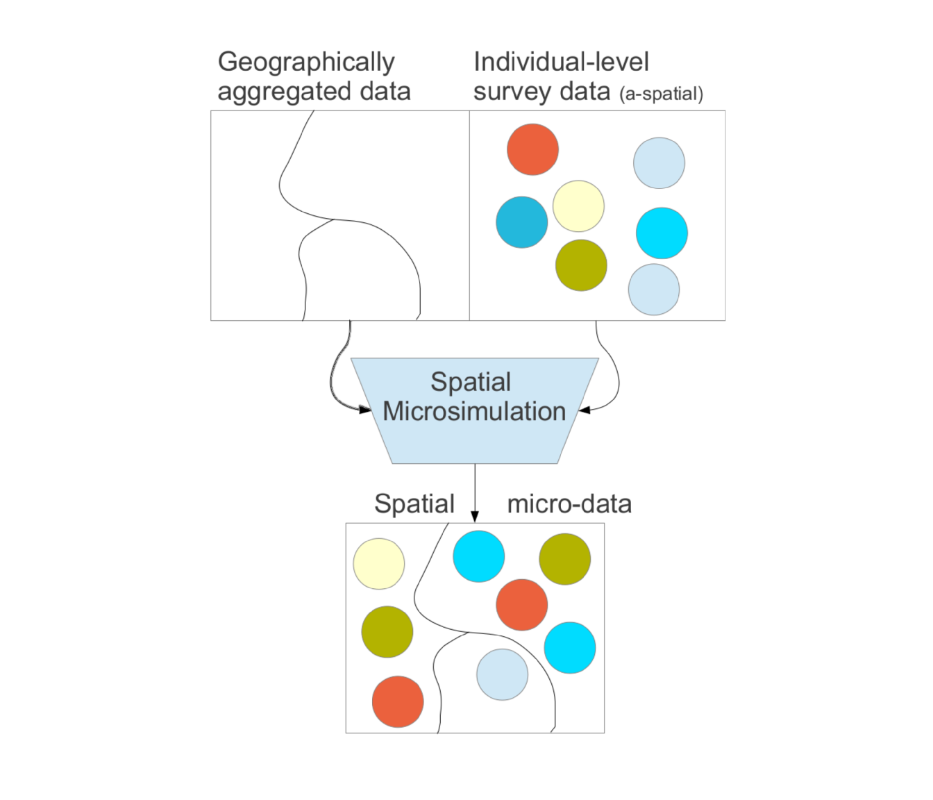
Figure 1.1: Schematic diagram contrasting conventional official data (above) against spatial microdata produced during population synthesis (below). Note that for brevity the geographically aggregated data are called constraints and the individual level survey data are called microdata in this book.
Throughout this book we use a broad definition of the term spatial microsimulation:
The creation, analysis and modelling of individual level data allocated to geographic zones.
To further clarify the distinction between the methodology and the approach, we use term population synthesis to describe the narrower process of generating the spatial microdata (see Chapter ). The term spatial microsimulation is reserved to describe the overall process, which usually involves population synthesis. Unless you are lucky enough to have access to real spatial microdata, a scarce but increasingly available commodity, spatial microdata must be generated by combining zone level and individual level data. Throughout the course of the book the emphasis shifts: the focus in Chapters 4 to 6 is on generating spatial microdata while Chapters 7 onwards focus on how to use this rich data type.
1.4 Learning by doing
Another issue tackled in this book is reproducibility, which is intimately linked to the ‘learning by doing’ approach. Notwithstanding a few exceptions (e.g. Williamson 2007), most findings in the field cannot be replicated: there is no way of independently verifying the results of spatial microsimulation research. Some model-based decisions, such as where to build smoking cessation clinics (Tomintz, Clarke, and Rigby 2008), are a matter of life or death. In such cases model transparency becomes vital.
Today fast internet connections, open access datasets and free software make it easier than ever to create reproducible research. This movement is growing in many fields, from Regional Science to Epidemiology (Ince, Hatton, and Graham-Cumming 2012; Peng, Dominici, and Zeger 2006; McNutt 2014; Rey 2014).
This book encourages ‘Open Science’ throughout. Reproducibility is encouraged through the provision of code. You will be expected to do spatial microsimulation rather than simply watch the results that others have produced! Small datasets are provided on which these ‘code chunks’ (such as that presented below) can run. All the findings presented in this book can therefore be reproduced using code and data in the book’s GitHub repository.
# This is a code chunk. Below is the code!
ind <- read.csv("data/SimpleWorld/ind-full.csv") # read-in data
print(ind[1,]) # print the 1st line of the data
## id age sex income
## 1 1 59 m 2868Notice that in addition to showing what to type into R, we show what the output should be. In fact, using the ‘RMarkdown’ file format, the code runs every time the book is compiled, ensuring the code’s long-term viability. There are good reasons to ensure such a reproducible work-flow. First, reproducibility can save time. Reproducible code that can be re-used multiple times, meaning you only have to write it once, reducing the need to ‘re-invent the wheel’ for every new analysis. Second, reproducibility can increase research impact: by enabling and encouraging others to use your work, it can gain more credit and, if you are in academia, citations. The third reason is more profound: reproducibility is a prerequisite of falsifiability, the backbone of science (Popper 1959). The results of non-reproducible research cannot be verified, reducing its scientific credibility. All these reasons inform the book’s practical nature.
This book presents spatial microsimulation as a living, evolving set of techniques rather than a prescriptive formula for arriving at the ‘right’ answer. Spatial microsimulation is largely defined by its user-community, made up of a growing number of people worldwide. This book aims to contribute to the community by encouraging collaboration, innovation and rigour. It also encourages playing with the methods and ‘getting your hands dirty’ with the code. As Kabacoff (2011, xxii) put it regarding R: “The best way to learn is to experiment”.
1.5 Why spatial microsimulation with R?
Software decisions have a major impact on the flexibility, efficiency and reproducibility of research. Nearly three decades ago Clarke and Holm (1987) observed that “little attention is paid to the choice of programming language used” for microsimulation. This appears to be as true now as it was then. Software is rarely discussed in papers on the subject and there are few mature spatial microsimulation packages.1 There is a strong and diverse software community in the ABM field, and many of these bring insights that could be of use to researchers using spatial microsimulation. Mannion et al. (2012), for example, present JAMSIM. This is a new software framework for combining the powerful Repast ABM application with R for graphing and analysis of the results. JAMSIM and other projects in the field (including the development of NetLogo and MASON ABM systems and associated add-ons) should be seen as developing in parallel to the R approach developed in this field, not competitors. There is clearly much potential for mutual benefit by software for ABM and spatial microsimulation interacting more closely together.
Factors that should influence software selection include cost, maturity, features and performance. Perhaps most important for busy researchers are the ease and speed of learning, writing, adapting and communicating the analysis. R excels in each of these areas.
R is a low level language compared with statistical programs based on a strong graphical user interface (GUI) such as Microsoft Excel and SPSS. R offers great flexibility for analysing and modelling data and enables easy creation of user-defined functions. These are all desirable attributes of software for undertaking spatial microsimulation. On the other hand, R is high level compared with general purpose languages such as C and Python. Instead of writing code to perform statistical operations ‘from scratch’, R users generally use pre-made functions. To calculate the mean value of variable x, for example, one would need to type 20 characters in Python: float(sum(x))/len(x).2 In pure R just 7 characters are sufficient: mean(x). This terseness and range of pre-made functions is useful for ease of reading and writing spatial microsimulation models and analysing the results.
The example of calculating the mean in R and Python may be trite but illustrates a wider point: R was designed to work with statistical data, so many functions in the default R installation (e.g. lm(), to create a linear regression model) perform statistical analysis ‘out of the box’. In agent-based modelling, the statistical analysis of results often occupies more time than running the model itself (Thiele, Kurth, and Grimm 2014). The same applies to spatial microsimulation, making R an ideal choice due to its statistical analysis capabilities.
R has an active and growing user community and is easy to extend. R’s extreme flexibility allows it to call code written in other programming languages. This means that ‘glass ceilings’ encountered in other environments are not an issue in R: there is a wide range of algorithms that can be used from within R. This ability has been used to dramatically speed up R code. The new R package dplyr, for example, uses C++ code to do the hard work of data manipulation tasks.
As a result of R’s flexibility, open source ethic and strong user community, there are thousands of packages that extend R’s capabilities with new functions. Improvements are being added to the ‘R ecosystem’ all the time. This book provides an overview of the functionality of key packages for spatial microsimulation. Software development is a fast moving game, however, so keep a look out for updates. New software can save both research and computer time so it’s worth staying up-to-date with the latest developments.
The ipfp and mipfp packages, for example, can greatly reduce the number of lines of code and the computational time needed for population synthesis compared with ‘hard-coding’ the method in R from scratch. (For the curious reader, the ‘IPF’ letters in the package names stand for ‘Iterative Proportional Fitting’, one of a number of technical terms we will use frequently in subsequent chapters. See the Glossary for a definition.)
These time-saving add-ons to R are described in Chapter 5. A clear advantage of R is that anyone can write a package. This is also potentially a disadvantage: it has been argued there are too many packages, making it difficult for new users to identify which packages are most reliable and which are best suited to different situations (Hornik 2012). However, this problem is mitigated by the open-source nature of R: users can see precisely how any particular function works (providing they are willing to learn some programming), rather than relying on a “black box”.
A recent development that has made R far more accessible is RStudio, an Integrated Development Environment (IDE) for R that helps new users become familiar with the language (see Figure 2.2). Further information about why R is a good choice for spatial microsimulation is provided in the Appendix, a tutorial introduction to R for spatial microsimulation applications. The next section describes approaches to learning R in general terms.
1.6 Learning the R language
Having learned a little about why R is a good tool for the job, it is worth considering at this stage how R should be used. It is useful to think of R not as a series of isolated commands, but as an interconnected language. The code is used not only for the computer to crunch numbers, but also to communicate ideas, from one person to another. In other words, this book teaches spatial microsimulation in the language of R. Of course, English is more appropriate than R for explaining rather than merely describing the method and the language of mathematics is ideal for describing quantitative relationships conceptually. However, because the practical components of this book are implemented in R, you will gain more from it if you are fluent in R. To this end the book aims to improve your R skills as well as your ability to perform spatial microsimulation, especially in the earlier practical chapters. Some prior knowledge of R will make reading this book easier, but R novices should be able to follow the worked examples, with reference to appropriate supplementary material.
The references listed in the Appendix () provide a recommended starting point for R novices. For complete beginners, we recommend the introductory ‘Owen R Guide’ (Owen 2006). As with learning Spanish or Chinese, frequent practice, persistence and experimentation will ensure deep learning.
A more practical piece of advice is to organise your workflow. Each project should have its own self-contained folder containing all that is needed to replicate the analysis, except perhaps large input datasets. This could include the raw (unchanged) input data3, R code for analysis, the graphical outputs and files containing data outputs. To avoid clutter, it is sensible to arrange this content into folders, as illustrated below (thanks to Colin Gillespie for this tip):
|-- book.Rmd
|-- data
|-- figures
|-- output
|-- R
|   |-- load.R
|   `-- parallel-ipfp.R
`-- spatial-microsim-book.Rproj
The example directory structure above is taken from an early version of this book. It contains the document for the write-up (book.Rmd — this could equally be a .docx or .tex file) and RStudio’s .Rproj file in the source directory. The rest of the entities are folders: one for the input data, one for figures generated, one for data outputs and one for R scripts. The R scripts should have meaningful names and contain only code that works and is commented. An additional backup directory could be used to store experimental code. There is no need to be prescriptive in following this structure, but projects using spatial microdata tend to be complex, so imposing order over your workflow early will likely yield dividends in the long run. If you work in a team, this kind of structure helps each member to rapidly understand and continue your work.
The same applies to learning the R language. Fluency allows complex numerical ideas to be described with a few keystrokes. If you are a new R user it is therefore worth spending some time learning the R language. To this end the Appendix provides a primer on R from the perspective of spatial microsimulation.
1.7 Typographic conventions
The following typographic conventions are followed to make the practical examples easier to follow:
- In-line code is provided in
monospacefont to show it’s something the computer understands. - Larger blocks of code, referred to as listings, are provided on separate lines and have coloured syntax highlighting to distinguish between values, names and functions:
x <- c(1, 2, 5, 10) # create a vector
sqrt(x) # find the square root of x
## [1] 1.000000 1.414214 2.236068 3.162278- Output from the R console is preceded by the
##symbol, as illustrated above. - Comments are preceded by a single
#symbol to explain specific lines. - Often, reference will be made to files contained within the book’s project folder. The notation used to refer to the location of these files follows the way we refer to files and folders on Linux computers. Thus ‘code/CakeMap.R’ refers to a file titled ‘CakeMap.R’, within the ‘R’ directory of the project’s folder.
There are many ways to write R code that will generate the same results. However, to ensure clarity and consistency, a single style, advocated in a chapter in Hadley Wickham’s Advanced R, is followed throughout (Wickham 2014a). Consistent style and plentiful comments will make your code readable by yourself and others for decades to come.
1.8 An overview of the book
The book’s chapters progress in a logical order that corresponds to the steps typically taken during a spatial microsimulation research project that generates, analyses and models spatial microdata. The next two chapters are primarily conceptual, introducing the concept and applications of spatial microsimulation in more detail whilst the remaining chapters are practical. Because we’ll be making heavy use of terminology specific to spatial microsimulation, it is recommended that you read these introductory chapters before tackling the practical section that follow although this is not essential. If any of the words do not make sense, the Glossary at the end of the book may help to clarify what they mean.
In Part II, Chapters 4, 5, 6 and 7 cover in detail the process of population synthesis whereby spatial microdata is generated. This process is key to much spatial microsimulation work. These chapters should ideally be read together in that order, although Chapter 5 is the most important and provides the basics needed to create spatial microdata. Chapters 8 introduces the important step of model validation.
In Part III, Chapters 9 and 10 cover more advanced methods for generating spatial microdata when no individual level data is available and when household level data are required. These chapters are more self-standing and can be read in any order. The chapter titles and brief descriptions of their contents are as follows:
SimpleWorld is a simple and reproducible explanation of spatial microsimulation with reference to an imaginary planet. It’s also a chance to set up your system and RStudio settings to get the most out of the subsequent chapters.
What is spatial microsimulation? introduces the concepts and applications of spatial microsimulation not only as a narrow methodology but as an approach to understanding real-world phenomena.
Data preparation is dedicated to the boring but vital task of loading and ‘cleaning’ the input data, ready for spatial microsimulation.
Population synthesis uses the input data created in the previous chapter to perform population synthesis, the process of creating synthetic spatial microdata. The chapter describes the main functions and techniques that are used for undertaking this key aspect of spatial microsimulation, with a focus on the ipfp and mipfp packages, which perform Iterative Proportion Fitting (IPF).
Alternative approaches to population synthesis describes some alternative methods, beyond IPF, for population synthesis. These include an R implementation the Generalized Regression Weighting procedure (GREGWT), a description of ‘simulated annealing’ and a demonstration that population synthesis can be interpreted as a constrained optimisation problem. This final insight has the consequence that many previously developed optimisation algorithms can be used to perform the ‘heavy lifting’ of population synthesis. A few of these, including R’s
optimandGenSAfunctions, are tested, illustrating the importance of performance testing.Spatial microsimulation in the wild is based on a larger and more complex example than SimpleWorld called CakeMap, that uses real data. This chapter combines geographic constraints with non-geographical survey data to estimate the geographical variation in cake consumption.
Model checking and evaluation tackles the understudied but important questions of ‘is the model working?’ and ‘do the results coincide with reality?’. Here you will learn appropriate tests and checks to verify spatial microsimulation outputs and think about its underlying assumptions.
Population synthesis without microdata gives a way to produce a spatial microsimulation without having individual level data.
Household allocation explains techniques to group the synthetic individuals into households.
The TRESIS approach to spatial microsimulation describes an alternative approach to spatial microsimulation that operates at the household level. This contributed chapter, by Richard Ellison and David Hensher, demonstrates the population synthesis stage of the wider Transport and Environment Strategy Impact Simulator (TRESIS) modelling system.
Spatial microdata in agent-based models describes how the output from spatial microsimulation can be used as an input into more complex models.
The final thing to say in this opening chapter relates to the future of this book as an up-to-date and accessible teaching resource. Spatial Microsimulation with R is both a book and an open source, open access project that is designed to be improved on and updated by the authors and the community using spatial microsimulation. Any comments relating to code, content or clarity of explanation will therefore be gratefully received.4
References
Lovelace, Robin, and Ian Philips. 2014. “The ‘oil vulnerability’ of commuter patterns: A case study from Yorkshire and the Humber, UK.” Geoforum 51 (0): 169–82. doi:http://dx.doi.org/10.1016/j.geoforum.2013.11.005.
Deming, WE, and Frederick F Stephan. 1940. “On a least squares adjustment of a sampled frequency table when the expected marginal totals are known.” The Annals of Mathematical Statistics. http://www.jstor.org/stable/10.2307/2235722.
Clarke, Martin, and Einar Holm. 1987. “Microsimulation methods in spatial analysis and planning.” Geografiska Annaler. Series B. Human Geography 69 (2): 145–64. http://www.jstor.org/stable/10.2307/490448 http://www.jstor.org/stable/490448.
Williamson, Paul. 2007. “CO Instruction Manual: Working Paper 2007/1 (v. 07.06.25).” Vol. 1. University of Liverpool.
Tomintz, Melanie N M.N., Graham P Clarke, and Janette E J.E. Rigby. 2008. “The geography of smoking in Leeds: estimating individual smoking rates and the implications for the location of stop smoking services.” Area 40 (3). Wiley Online Library: 341–53.
Ince, Darrel C, Leslie Hatton, and John Graham-Cumming. 2012. “The case for open computer programs.” Nature 482 (7386). Nature Publishing Group: 485–8. doi:10.1038/nature10836.
Peng, Roger D., Francesca Dominici, and Scott L. Zeger. 2006. “Reproducible epidemiologic research.” American Journal of Epidemiology 163 (9): 783–9. doi:10.1093/aje/kwj093.
McNutt, Marcia. 2014. “Journals unite for reproducibility.” Science 346 (6210): 679. doi:10.1126/science.aaa1724.
Rey, Sergio J. 2014. “Open regional science.” The Annals of Regional Science 52 (3): 825–37. doi:10.1007/s00168-014-0611-7.
Popper, Karl. 1959. The Logic of scientific discovery. Hutchinson.
Kabacoff, Robert. 2011. R in Action. Manning Publications Co.
Mannion, Oliver, Roy Lay-Yee, Wendy Wrapson, Peter Davis, and Janet Pearson. 2012. “JAMSIM: A microsimulation modelling policy tool.” Journal of Artificial Societies and Social Simulation 15 (1): 8.
Thiele, JC, W Kurth, and V Grimm. 2014. “Facilitating Parameter Estimation and Sensitivity Analysis of Agent-Based Models: A Cookbook Using NetLogo and’R’.” Journal of Artificial Societies and … 17 (11).
Hornik, Kurt. 2012. “Are There Too Many R Packages?” Austrian Journal of Statistics 41 (1): 59–66.
Owen, WJ. 2006. “The R Guide.” Comprehensive R Archive Network.
Wickham, Hadley. 2014a. Advanced R. CRC Press.
The Flexible Modelling Framework (FMF) is a notable exception written in Java that can perform various modelling tasks.↩
The
floatfunction is needed in case integers are used. This can be reduced to 13 characters with the excellent NumPy package:import numpy; x = [1,3,9]; numpy.mean(x)would generate the desired result. The R equivalent isx = c(1,3,9); mean(x).↩Raw data should be kept safely on an external hard disk or a server if it is large or sensitive.↩
Feedback can be left via email to r.lovelace@leeds.ac.uk or via the project’s GitHub page (http://github.com/Robinlovelace/spatial-microsim-book).↩