5 Population synthesis

In this chapter we progress from loading and preparing the input data to running a spatial microsimulation model. The focus is on Iterative Proportional Fitting procedure (IPF), a simple, fast and widely-used method to allocate individuals to zones. Other methods can achieve the same result, as discussed in the first section of this chapter and as demonstrated in @ref(#alternative-reweighting).

This chapter moves from theory to practice. It describes the process underlying the method of population synthesis (Section 5.2.1) before implementing the IPF algorithm in base R (Section5.2.2). In the following sections two packages that automate IPF, ipfp and mipfp, are introduced (@ref(#ipfp) and @ref(#mipfp) respectively). The chapter also introduces the important concepts of integerisation and expansion. These methods are introduced towards the end of each package-specific section. The final section () compares the relative merits of ipfp and mipfp.

The SimpleWorld data, loaded in the previous chapter, is used as the basis of this chapter. Being small, simple and hopefully by now familiar, SimpleWorld facilitates understanding of the process on a ‘human scale’. As always, we encourage experimentation with small datasets to avoid the worry of overloading your computer, before applying the same methods to larger and more complex data. Learning the basic principles and methods of spatial microsimulation in R is the focus of this chapter. Time spent mastering these basics will make subsequent steps much easier.

How representative each individual is of each zone is represented by their weight for that zone. Each weight links an individual to a zone. The number of weights is therefore equal to the number of zones multiplied by the number of individuals in the microdata. In terms of the SimpleWorld data loaded in the previous chapter we have, in R syntax, nrow(cons) zones and nrow(ind) individuals (typing those commands with the data loaded should confirm that there are 3 zones and 5 individuals in the input data for the SimpleWorld example). This means that nrow(cons) * nrow(ind) weights will be estimated (that is \(3 * 5 = 15\) in SimpleWorld). The weights must begin with an initial value. We will create a matrix of ones. Thus, every individual is seen as equally representative of every zone:¹⁴

# Create the weight matrix. 
# Note: relies on data from previous chapter.
weights <- matrix(data = 1, nrow = nrow(ind), ncol = nrow(cons))
dim(weights) # dimension of weight matrix: 5 rows by 3 columns

## [1] 5 3

The weight matrix links individual level data to aggregate level data. A weight matrix value of 0 in cell [i,j], for example, suggests that the individual i is not representative of zone j. During the IPF procedure these weights are iteratively updated until they converge towards a single result: the final weights which create a representative population for each zone.¹⁵

5.1 Weighting algorithms

A wide range of methods can be used to allocate individuals to zones in spatial microsimulation. As with the majority of procedures for statistical analysis, there are deterministic and stochastic methods. The results of deterministic methods, such as IPF, never vary: no random or probabilistic numbers are used so the resulting weights will be the same every time. Stochastic methods such as simulated annealing, on the other hand, use some random numbers.

In the literature, the divide between stochastic and deterministic approaches is usually mapped onto a wider distinction between reweighting and combinatorial optimisation methods. Reweighting methods generally calculate non-integer weights for every individual-zone combination. Combinatorial optimisation methods generally work by randomly allocating individuals from the microdata survey into each zone, one-by-one, and re-calculating the goodness-of-fit after each change. If the fit between observed and simulated results improves after an individual has been ‘imported’ into the zone in question, the individual will stay. If the fit deteriorates, the individual will be removed from the zone and the impact of switching a different individual into the zone is tested.

This distinction between reweighting of fractional weights and combinatorial optimisation algorithms is important: combinatorial optimisation methods result in whole individuals being allocated to each zone whereas reweighting strategies result in fractions of individuals being allocated to each zone. The latter method means that individual \(i\) could have a weight of 0.223 (or any other positive real number) for zone \(j\). Of course, this sounds irrational: a quarter of a person cannot possibly exist: either she is in the zone or she is not!

However, the distinction between combinatorial optimisation and reweighting approaches to creating spatial microdata is not as clear cut as it may at first seem. As illustrated in Figure 5.1, fractional weights generated by reweighting algorithms such as IPF can be converted into integer weights (via integerisation).

Through the process of expansion, the integer weight matrix produced by integerisation can be converted into the final spatial microdata output stored in ‘long’ format represented in the right-hand box of Figure~5.1. Thus the combined processes of integerisation and expansion allow weight matrices to be translated into the same output format that combinatorial optimisation algorithms produce directly. In other words fractional weighting is interchangeable with combinatorial optimisation approaches for population synthesis.

The reverse process is also possible: synthetic spatial microdata generated by combinatorial optimisation algorithms can be converted back in to a more compact weight matrix in a step that we call compression. This integer weight has the same dimensions as the integer matrix generated through integerisation described above.

Integerisation, expansion and compression procedures allow fractional weighting and combinatorial optimisation approaches for population synthesis to be seen as essentially the same thing.

This equivalence between different methods of population synthesis is the reason we have labelled this section weighting algorithms: combinatorial optimisation approaches to population synthesis can be seen as a special case of fractional weighting and vice versa. Thus all deterministic and stochastic (or weighting and combinatorial optimisation) approaches to the generation of spatial microdata can be seen as different methods, algorithms, for allocating weights to individuals. Individuals representative of a zone will be given a high weight (which is equivalent to being replicated many times in combinatorial optimisation). Individuals who are rare in a zone will be given a low weight (or not appear at all, equivalent to a weight of zero). Later in this chapter we demonstrate functions to translate between the ‘weight matrix’ and ‘long spatial microdata’ formats generated by each approach.

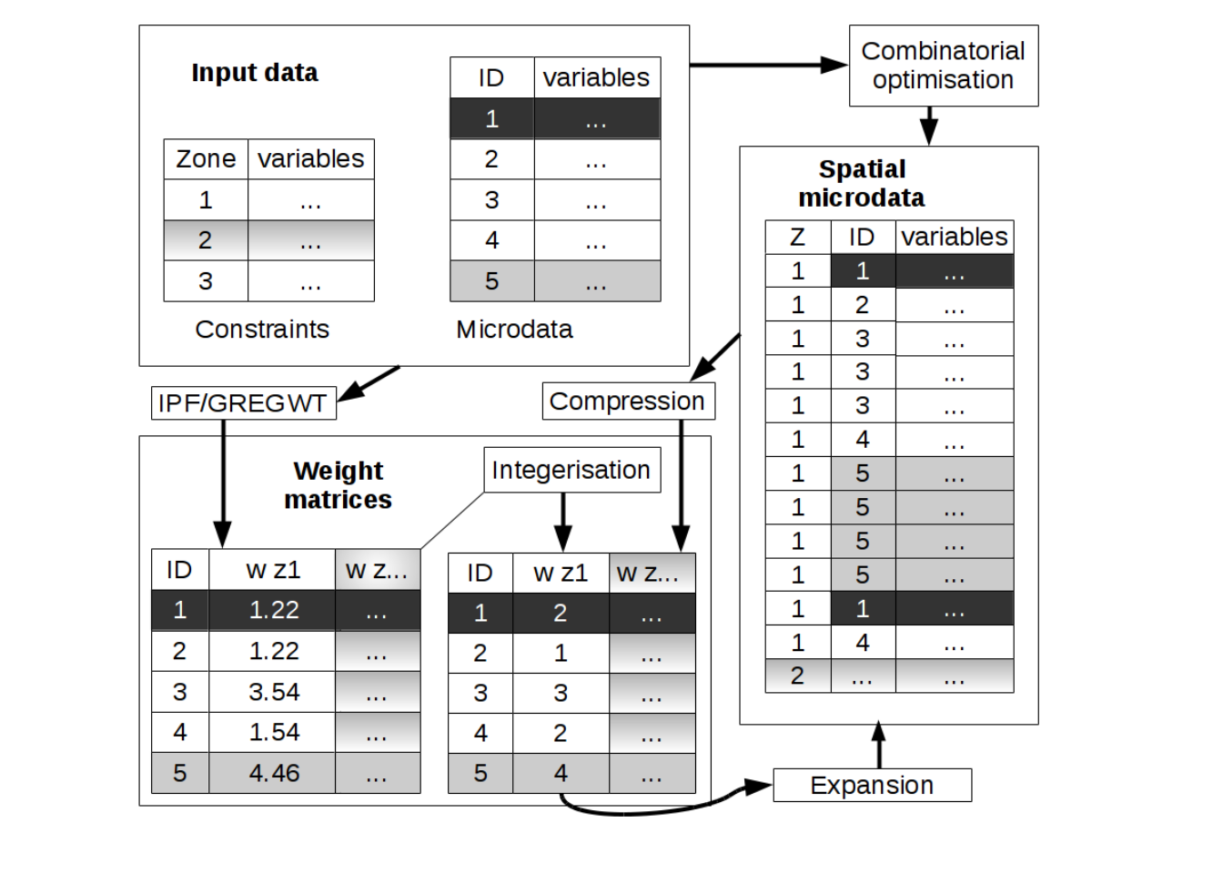
Figure 5.1: Schematic of different approaches for the creation of spatial microdata encapsulating stochastic combinatorial optimisation and deterministic reweighting algorithms such as IPF. Note that integerisation and ‘compression’ steps make the results of the two approaches interchangeable, hence our use of the term ‘reweighting algorithm’ to cover all methods for generating spatial microdata.

The concept of weights is critical to understanding how population synthesis generates spatial microdata. To illustrate the point imagine a parallel SimpleWorld, in which we have no information about the characteristics of its inhabitants, only the total population of each zone. In this case we could only assume that the distribution of characteristics found in the sample is representative of the distribution of the whole population. Under this scenario, individuals would be chosen at random from the sample and allocated to zones at random and the distribution of characteristics of individuals in each zone would be asymptotically the same as (tending towards) the microdata.

In R, this case can be achieved using the sample() command. We could use this method to randomly allocate the 5 individuals of the microdata to zone 1 (which has a population of 12) with the following code:

# set the seed for reproducibility
set.seed(1) 
# create selection
sel <- sample(x = 5, size = 12, replace = T)
ind_z1 <- ind_orig[sel, ]
head(ind_z1, 3)

##     id age sex income
## 2    2  54   m   2474
## 2.1  2  54   m   2474
## 3    3  35   m   2231

Note the use of set.seed() in the above code to ensure the results are reproducible. It is important to emphasise that without ‘setting the seed’ (determining the starting point of the random number sequence) the results will change each time the code is run. This is because sample() (along with other stochastic functions such as runif() and rnorm()) is probabilistic and its output therefore depends on a random number generator (RNG).¹⁶

The reweighting methods consists in adding a weight to each individual for the zone. This method is good if we have a representative sample of the zone and the minority of the population is included in it. In contrary, if we have in the individual level only the majority of the population and for example, we have not an old man still working, this kind of individual will not appear in the final data. A proposal to avoid this is to either modify the sample to include those outliers or use a different approach such as a genetic algorithm to allow mixing some individual level variables to create a new individuals (mutation). We are not aware of the latter technique being used at present, although it could be used in future microsimulation work. An other useful alternative to solve this issue is given by the tabu-search algorithm, an heuristic for integer programming method. (Glover 1986, 1989, 1990 and Glover and Laguna, 1997). This heuristic can be used to improve an initial solution produced by the IPF.

In the rest of this chapter, we develop an often used reweighting algorithm : the Iterative Proportional Fitting (IPF). When reweighting, three steps are always necessary. First, you generate a weight matrix containing fractional numbers, then you integerise it. When knowing the number of times each individual needs to be replicated, the expansion step calculates the final dataset, which contains a row per individual in the whole population and a zone for each person. The process is explained in theory and then demonstrated with example code in R.

5.2 Iterative Proportional Fitting

This section begins with the theory (and intuition) under the IPF algorithm. Then, the R code to run the method is explained. However, in R, it is often unnecessary to write the whole code. Indeed, packages including functions to perform an IPF exist and are optimised. The ipfp and mipfp packages are the subjects of the two last sub-sections of this section.

5.2.1 IPF in theory

The most widely used and mature deterministic method to allocate individuals to zones is iterative proportional fitting (IPF). IPF is mature, fast and has a long history: it was demonstrated by Deming and Stephan (1940) for estimating internal cells based on known marginals. IPF involves calculating a series of non-integer weights that represent how representative each individual is of each zone. This is reweighting.

Regardless of implementation method, IPF can be used to allocate individuals to zones through the calculation of maximum likelihood values for each zone-individual combination represented in the weight matrix. This is considered as the most probable configuration of individuals in these zones. IPF is a method of entropy maximisation (Cleave et al. 1995). The entropy is the number of configurations of the underlying spatial microdata that could result in the same marginal counts. For in-depth treatment of the mathematics and theory underlying IPF, interested readers are directed towards Fienberg (1979), Cleave et al. (1995) and an excellent recent review of methods for maximum likelihood estimation (Fienberg and Rinaldo 2007). For the purposes of this book, we provide a basic overview of the method for the purposes of spatial microsimulation.

In spatial microsimulation, IPF is used to allocate individuals to zones. The subsequent section implements IPF to create spatial microdata for SimpleWorld, using the data loaded in the previous chapter as a basis. An overview of the paper from the perspective of transport modelling is provided by Pritchard and Miller (2012).

Such as with the example of SimpleWorld, each application has a matrix ind containing the categorical value of each individual. ind is a two dimensional array (a matrix) in which each row represents an individual and each column a variable. The value of the cell ind(i,j) is therefore the category of the individual i for the variable j.

A second array containing the constraining count data cons can, for the purpose of explaining the theory, be expressed in three dimensions, which we will label cons_t: cons_t(i,j,k) is the number of individuals corresponding to the marginal for the zone ‘i’, in the variable ‘j’ for the category ‘k’. For example, ‘i’ could be a municipality, ‘j’ the gender and ‘k’ the female. Element ‘(i,j,k)’ is the total number of women in this municipality according to the constraint data.

The IPF algorithm will proceed zone per zone. For each zone, each individual will have a weight of ‘representatively’ of the zone. The weight matrix will then have the dimension ‘number of individual x number of zone’. ‘w(i,j,t)’ corresponds to the weight of the individual ‘i’ in the zone ‘j’ (during the step ‘t’). For the zone ‘z’, we will adapt the weight matrix to each constraint ‘c’. This matrix is initialized with a full matrix of 1 and then, for each step ‘t’, the formula can be expressed as:

\[ w(i,z,t+1) = w(i,z,t) * \displaystyle\frac{cons \_ t(z,c,ind(i,c))}{ \displaystyle\sum_{j=1}^{n_{ind}} w(j,z,t) * I(ind(j,c)=ind(i,c))} \]

where the ‘I(x)’ function is the indicator function which value is 1 if x is true and 0 otherwise. We can see that ‘ind(i,c)’ is the category of the individual ‘i’ for the variable ‘c’. The denominator corresponds to the sum of the actual weights of all individuals having the same category in this variable as ‘i’. We simply redistribute the weights so that the data follows the constraint concerning this variable.

5.2.2 IPF in R

In the subsequent examples, we use IPF to allocate individuals to zones in SimpleWorld, using the data loaded in the previous chapter as a basis. IPF is mature, fast and has a long history.

The IPF algorithm can be written in R from scratch, as illustrated in Lovelace (2014), and as taught in the smsim-course on-line tutorial. We will refer to this implementation of IPF as ‘IPFinR’. The code described in this tutorial ‘hard-codes’ the IPF algorithm in R and must be adapted to each new application (unlike the generalized ‘ipfp’ approach, which works unmodified on any reweighting problem). IPFinR works by saving the weight matrix after every constraint for each iteration. We here develop first IPFinR to give you an idea of the algorithm. Without reading the source code in the ipfp and mipfp packages, available from CRAN, they can seem like “black boxes” which magically generate answers without explanation of how answer was created.

By the end of this section you will have generated a weight matrix representing how representative each individual is of each zone. The algorithm operates zone per zone and the weight matrix will be filled in column per column. For convenience, we begin by assigning some of the basic parameters of the input data to intuitive names, for future reference.

# Create intuitive names for the totals
n_zone <- nrow(cons) # number of zones
n_ind <- nrow(ind) # number of individuals
n_age <-ncol(con_age) # number of categories of "age"
n_sex <-ncol(con_sex) # number of categories of "sex"

The next code chunk creates the R objects needed to run IPFinR. The code creates the weight matrix (weights) and the marginal distribution of individuals in each zone (ind_agg0). Thus first we create an object (ind_agg0), in which rows are zones and columns are the different categories of the variables. Then, we duplicate the weight matrix to keep in memory each step.

# Create initial matrix of categorical counts from ind 
weights <- matrix(data = 1, nrow = nrow(ind), ncol = nrow(cons))
# create additional weight objects
weights1 <- weights2 <- weights 
ind_agg0 <- t(apply(cons, 1, function(x) 1 * ind_agg))
colnames(ind_agg0) <- names(cons)

IPFinR begins with a couple of nested ‘for’ loops, one to iterate through each zone (hence 1:n_zone, which means “from 1 to the number of zones in the constraint data”) and one to iterate through each category within the constraints (0–49 and 50+ for the first constraint), using the cons and ind objects loaded in the previous chapter.

# Assign values to the previously created weight matrix 
# to adapt to age constraint
for(j in 1:n_zone){
  for(i in 1:n_age){
    index <- ind_cat[, i] == 1
    weights1[index, j] <- weights[index, j] * con_age[j, i] 
    weights1[index, j] <- weights1[index, j] / ind_agg0[j, i]
    }
  print(weights1)
}

##          [,1] [,2] [,3]
## [1,] 1.333333    1    1
## [2,] 1.333333    1    1
## [3,] 4.000000    1    1
## [4,] 1.333333    1    1
## [5,] 4.000000    1    1
##          [,1]     [,2] [,3]
## [1,] 1.333333 2.666667    1
## [2,] 1.333333 2.666667    1
## [3,] 4.000000 1.000000    1
## [4,] 1.333333 2.666667    1
## [5,] 4.000000 1.000000    1
##          [,1]     [,2]     [,3]
## [1,] 1.333333 2.666667 1.333333
## [2,] 1.333333 2.666667 1.333333
## [3,] 4.000000 1.000000 3.500000
## [4,] 1.333333 2.666667 1.333333
## [5,] 4.000000 1.000000 3.500000

The above code updates the weight matrix by multiplying each weight by a coefficient to respect the desired proportions (age constraints). These coefficients are the divisions of each cell in the census constraint (con_age) by the equivalent cell aggregated version of the individual level data. In the first step, all weights were initialised to 1 and the new weights equal the coefficients. Note that the two lines changing weights1 could be joined to form only one line (we split it into two lines to respect the margins of the book). The weight matrix is critical to the spatial microsimulation procedure because it describes how representative each individual is of each zone. To see the weights that have been allocated to individuals to populate, for example zone 2, you would query the second column of the weights: weights1[, 2]. Conversely, to see the weight allocated for individual 3 for each for the 3 zones, you need to look at the 3rd column of the weight matrix: weights1[3, ].

Note that we asked R to write the resulting matrix after the completion of each zone. As said before, the algorithm proceeds zone per zone and each column of the matrix corresponds to a zone. This explains why the matrix is filled in per column. We can now verify that the weights correspond to the application of the theory seen before.

For the first zone, the age constraint was to have 8 people under 50 years old and 4 over this age. The first individual is a man of 59 years old, so over 50. To determine the weight of this person inside the zone 1, we multiply the actual weight, 1, by a ratio with a numerator corresponding to the number of persons in this category of age for the constraint, here 4, and a denominator equal to the sum of the weights of the individual having the same age category. Here, there are 3 individuals of more than 50 years old and all weights are 1 for the moment. The new weight is \[ 1 * \frac{4}{1+1+1}=1.33333\] We can verify the other weights with a similar reasoning. Now that we explained the whole process under IPF, we can understand the origin of the name ‘Iterative Proportional Fitting’.

Thanks to the weight matrix, we can see that individual 3 (whose attributes can be viewed by entering ind[3, ]) is young and has a comparatively low weight of 1 for zone two. Intuitively this makes sense because zone 2 has only 2 young adult inhabitants (see the result of cons[2,]) but 8 older inhabitants. The reweighting stage is making sense. Note also that the weights generated are fractional; see 5.3 for methods of converting fractional weights into integer weights to generate a synthetic small-area population ready for agent-based modelling applications.

The next step in IPF, however, is to re-aggregate the results from individual level data after they have been reweighted. For the first zone, the weights of each individual are in the first column of the weight matrix. Moreover, the characteristics of each individual are inside the matrix ind_cat.

When multiplying ind_cat by the first column of weights1 we obtain a vector, the values of which correspond to the number of people in each category for zone 1. To aggregate all individuals for the first zone, we just sum the values in each category. The following for loop re-aggregates the individual level data, with the new weights for each zone:

# Create additional ind_agg objects
ind_agg2 <- ind_agg1 <- ind_agg0 * NA

# Assign values to the aggregated data after con 1
for(i in 1:n_zone){
  ind_agg1[i, ] <- colSums(ind_cat * weights1[, i])
}

If you are new to IPF, congratulations: you have just reweighted your first individual level dataset to a geographical constraint (the age) and have aggregated the results. At this early stage it is important to do some preliminary checks to ensure that the code is working correctly. First, are the resulting populations for each zone correct? We check this for the first constraint variable (age) using the following code (to test your understanding, try to check the populations of the unweighted and weighted data for the second constraint — sex):

rowSums(ind_agg1[, 1:2]) # the simulated populations in each zone

## [1] 12 10 11

rowSums(cons[, 1:2]) # the observed populations in each zone

## [1] 12 10 11

The results of these tests show that the new populations are correct, verifying the technique. But what about the fit between the observed and simulated results after constraining by age? We will cover goodness of fit in more detail in subsequent sections. For now, suffice to know that the simplest way to test the fit is by using the cor function on a 1d representation of the aggregate level data:

vec <- function(x) as.numeric(as.matrix(x))
cor(vec(ind_agg0), vec(cons))

## [1] -0.3368608

cor(vec(ind_agg1), vec(cons))

## [1] 0.628434

The point here is to calculate the correlation between the aggregate actual data and the constraints. This value is between -1 and 1 and in our case, the best fit will be 1, meaning that there is a perfect correlation between our data and the constraints. Note that as well as creating the correct total population for each zone, the new weights also lead to much better fit. To see how this has worked, let’s look at the weights generated for zone 1:

weights1[, 1]

## [1] 1.333333 1.333333 4.000000 1.333333 4.000000

The results mean that individuals 3 and 5 have been allocated a weight of 4 whilst the rest have been given a weight of \(4/3\). Note that the total of these weights is 12, the population of zone 1. Note also that individuals 3 and 5 are in the younger age group (verify this with ind$age[c(3,5)]) which are more commonly observed in zone 1 than the older age group:

cons[1, ]

##   a0_49 a50+ m f
## 1     8    4 6 6

Note there are 8 individuals under 50 years old in zone 1, but only 2 individuals with this age in the individual level survey dataset. This explains why the weight allocated to these individuals was 4: 8 divided by 2 = 4.

So far we have only constrained by age. This results in aggregate level results that fit the age constraint but not the sex constraint (Figure 5.2). The reason for this should be obvious: weights are selected such that the aggregated individual level data fits the age constraint perfectly, but no account is taken of the sex constraint. This is why IPF must constrain for multiple constraint variables.

To constrain by sex, we simply repeat the nested for loop demonstrated above for the sex constraint. This is implemented in the code block below.

for(j in 1:n_zone){
  for(i in 1:n_sex + n_age){
    index <- ind_cat[, i] == 1
    weights2[index, j] <- weights1[index, j] * cons[j , i] /
      ind_agg1[j, i]
    }
}

Again, the aggregate values need to be calculated in a for loop over every zone. After the first constraint fitting, the weights for zone 1 were:

\[(\frac{4}{3},\frac{4}{3},4,\frac{4}{3},4) \]

We can explain theoretically explain the weights for zone 1 after the second fitting. For the first individual, its actual weight is \(\frac{4}{3}\) and he is a male. In zone 1, the constraint is to have 6 men. The three first individuals are men, so the new weight for this person in this zone is \[weights2[1,1]=\frac{4}{3}*\frac{6}{\frac{4}{3}+\frac{4}{3}+4}=\frac{6}{5}=1.2 \]

With an analogous reasoning, we can find all weights in weights2:

weights2

##      [,1]      [,2]      [,3]
## [1,]  1.2 1.6842105 0.6486486
## [2,]  1.2 1.6842105 0.6486486
## [3,]  3.6 0.6315789 1.7027027
## [4,]  1.5 4.3636364 2.2068966
## [5,]  4.5 1.6363636 5.7931034

Note that the final value is calculated by multiplying by ind_cat and weights2.

for(i in 1:n_zone){
  ind_agg2[i, ] <- colSums(ind_cat * weights2[, i])
}

ind_agg2

##         a0_49     a50+ m f
## [1,] 8.100000 3.900000 6 6
## [2,] 2.267943 7.732057 4 6
## [3,] 7.495806 3.504194 3 8

Note that even after constraining by age and sex, there is still not a perfect fit between observed and simulated cell values (Figure 5.2). After constraining only by age, the simulated cell counts for the sex categories are far from the observed, whilst the cell counts for the age categories fit perfectly. On the other hand, after constraining by age and sex, the fit is still not perfect. This time the age categories do not fit perfectly, whilst the sex categories fit perfectly. Inspect ind_agg1 and ind_agg2 and try to explain why this is. The concept of IPF is to repeat this procedure several times. Thus, each iteration contains a re-constraining for each variable. In our case, the name iteration 1.1 and 1.2 describe the first iteration constrained only by age and then by sex, respectively. The overall fit, combining age and sex categories, has improved greatly from iteration 1.1 to 1.2 (from \(r = 0.63\) to \(r = 0.99\)). In iteration 2.1 (in which we constrain by age again) the fit improves again.

So, each time we reweight to a specific constraint, the fit of this constraint is perfect, because, as seen in theory, it is a proportional reallocation. Then, we repeat for another constraint and the first one can diverge from this perfect fit. However, when operating this process several times, we always refit to the next constraint and we can converge to a unique weight matrix.

## 
## Attaching package: 'tidyr'

## The following object is masked from 'package:mipfp':
## 
##     expand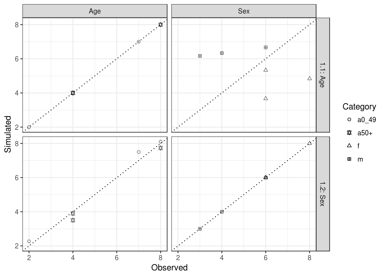

(#fig:valit_plot1)Fit between observed and simulated values for age and sex categories (column facets) after constraining a first time by age and sex constraints (iterations 1.1 and 1.2, plot rows). The dotted line in each plot represents perfect fit between the simulated and observed cell values. The overall fit in each case would be found by combining the left and right-hand plots. Each symbol corresponds to a category and each category has a couple (observed, simulated) for each zone.

These results show that IPF requires multiple iterations before converging on a single weight matrix. It is relatively simple to iterate the procedure illustrated in this section multiple times, as described in the smsim-course tutorial. However, for the purposes of this book, we will move on now to consider implementations of IPF that automate the fitting procedure and iteration process. The aim is to make spatial microsimulation as easy and accessible as possible.

The advantage of hard-coding the IPF process, as illustrated above, is that it helps understand how IPF works and aids the diagnosis of issues with the reweighting process as the weight matrix is re-saved after every constraint and iteration. However, there are more computationally efficient approaches to IPF. To save computer and researcher time, we use in the next sections R packages which implement IPF without the user needing to hard code each iteration in R: ipfp and mipfp. We will use each of these methods to generate fractional weight matrices allocating each individual to zones. After following this reweighting process with ipfp, we will progress to integerisation: the process of converting the fractional weights into integers. This process creates a final contingency table, which is used to generate the final population. This last step is called the expansion.

5.2.3 IPF with ipfp

IPF runs much faster and with less code using the ipfp package than in pure R. The ipfp function runs the IPF algorithm in the C language, taking aggregate constraints, individual level data and an initial weight vector (x0) as inputs:

library(ipfp) # load ipfp library after install.packages("ipfp")
cons <- apply(cons, 2, as.numeric) # to 1d numeric data type
ipfp(cons[1,], t(ind_cat), x0 = rep(1, n_ind)) # run IPF

## [1] 1.227998 1.227998 3.544004 1.544004 4.455996

It is impressive that the entire IPF process, which takes dozens of lines of code in base R (the IPFinR method), can been condensed into two lines: one to convert the input constraint dataset to numeric¹⁷ and one to perform the IPF operation itself. The whole procedure is hiding behind the function that is created in C and optimised. So, it is like a magic box where you put your data and that returns the results. This is a good way to execute the algorithm, but one must pay attention to the format of the input argument to use the function correctly. To be sure, type on R ?ipfp.

Note that although we did not specify how many iterations to run, the above command ran the default of maxit = 1000 iterations, despite convergence happening after 10 iterations. Note that ‘convergence’ in this context means that the norm of the matrix containing the difference between two consecutive iterations reaches the value of tol, which can be set manually in the function (e.g. via tol = 0.0000001). The default value of tol is .Machine$double.eps, which is a very small number indeed: 0.000000000000000222, to be precise.

The number of iterations can also be set by specifying the maxit argument (e.g. maxit = 5). The result after each iteration will be printed if we enable the verbose argument with verbose = TRUE. Note also that these arguments can be referred to lazily using only their first letter: verbose can be referred to as v, for example, as illustrated below (not all lines of R output are shown):

ipfp(cons[1,], t(ind_cat), rep(1, n_ind), maxit = 20, v = T)

## iteration 0:   0.141421
## iteration 1:   0.00367328
## iteration 2:   9.54727e-05
## ...
## iteration 9:   4.96507e-16
## iteration 10:  4.96507e-16

To be clear, the maxit argument in the above code specifies the maximum number of iterations and setting verbose to TRUE (the default is FALSE) instructed R to print the result. Being able to control R in this way is critical to mastering spatial microsimulation with R.

The numbers that are printed in the output from R correspond to the ‘distance’ between the previous and actual weight matrices. When the two matrices are equal, the algorithm has converged and the distance will approach 0. If the distance falls below the value of tol, the algorithm stops. Note that when calculating, the computer makes numerical approximations of real numbers. For example, when calculating the result of \(\frac{4}{3}\), the computer cannot save the infinite number of decimals and truncates the number.

Due to this, we rarely reach a perfect 0 but we assume that a result that is very close to zero is sufficient. Usually, we use the precision of the computer that is of order \(10^{-16}\) (on R, you can display the precision of the machine by typing .Machine$double.eps).

Notice also that for the function to work a transposed (via the t() function) version of the individual level data (ind_cat) was used. This differs from the ind_agg object used in the pure R version. To prevent having to transpose ind_cat every time ipfp is called, we save the transposed version:

ind_catt <- t(ind_cat) # save transposed version of ind_cat

Another object that can be saved prior to running ipfp on all zones (the rows of cons) is rep(1, nrow(ind)), simply a series of ones - one for each individual. We will call this object x0 as its argument name representing the starting point of the weight estimates in ipfp:

x0 <- rep(1, n_ind) # save the initial vector

To extend this process to all three zones we can wrap the line beginning ipfp(...) inside a for loop, saving the results each time into a weight variable we created earlier:

weights_maxit_2 <- weights # create a copy of the weights object
for(i in 1:ncol(weights)){
  weights_maxit_2[,i] <- ipfp(cons[i,], ind_catt, x0, maxit = 2)
}

The above code uses i to iterate through the constraints, one row (zone) at a time, saving the output vector of weights for the individuals into columns of the weight matrix. To make this process even more concise (albeit less clear to R beginners), we can use R’s internal for loop, apply:

weights <- apply(cons, MARGIN = 1, FUN = 
    function(x) ipfp(x, ind_catt, x0, maxit = 20))

In the above code R iterates through each row (hence the second argument MARGIN being 1, MARGIN = 2 would signify column-wise iteration). Thus ipfp is applied to each zone in turn, as with the for loop implementation. The speed savings of writing the function with different configurations are benchmarked in ‘parallel-ipfp.R’ in the ‘R’ folder of the book project directory. This shows that reducing the maximum iterations of ipfp from the default 1000 to 20 has the greatest performance benefit.¹⁸ To make the code run faster on large datasets, a parallel version of apply called parApply can be used. This is also tested in ‘parallel-ipfp.R’.

Take care when using maxit as the only stopping criteria as it is impossible to predict the number of iterations necessary to achieve the desired level of fit for every application. So, if your argument is too big you will needlessly lose time, but if it is too small, the result will not converge.

Using tol alone is also hazardous. Indeed, if you have iteratively the same matrices, but the approximations on the distance is a number bigger than your argument, the algorithm will continue. That’s why we use tol and maxit in tandem. Default values for maxit and tol are 1000 a very small number defined in R as .Machine$double.eps respectively.

It is important to check that the weights obtained from IPF make sense. To do this, we multiply the weights of each individual by rows of the ind_cat matrix, for each zone. Again, this can be done using a for loop, but the apply method is more concise:

ind_agg <- t(apply(weights, 2, function(x) colSums(x * ind_cat)))
colnames(ind_agg) <- colnames(cons) # make the column names equal

As a preliminary test of fit, it makes sense to check a sample of the aggregated weighted data (ind_agg) against the same sample of the constraints. Let’s look at the results (one would use a subset of the results, e.g. ind_agg[1:3, 1:5] for the first five values of the first 3 zones for larger constraint tables found in the real world):

ind_agg

##      a0_49 a50+ m f
## [1,]     8    4 6 6
## [2,]     2    8 4 6
## [3,]     7    4 3 8

cons

##      a0_49 a50+ m f
## [1,]     8    4 6 6
## [2,]     2    8 4 6
## [3,]     7    4 3 8

This is a good result: the constraints perfectly match the results generated using IPF, at least for the sample. To check that this is due to the ipfp algorithm improving the weights with each iteration, let us analyse the aggregate results generated from the alternative set of weights, generated with only 2 iterations of IPF:

# Update ind_agg values, keeping col names (note '[]')
ind_agg[] <- t(apply(weights_maxit_2, MARGIN = 2, 
  FUN = function(x) colSums(x * ind_cat)))
ind_agg[1:2, 1:4]

##         a0_49     a50+ m f
## [1,] 8.002597 3.997403 6 6
## [2,] 2.004397 7.995603 4 6

Clearly the final weights after 2 iterations of IPF represent the constraint variables well, but do not match perfectly except in the second constraint. This shows the importance of considering number of iterations in the reweighting stage — too many iterations can be wasteful, too few may result in poor results. To reiterate, 20 iterations of IPF are sufficient in most cases for the results to converge towards their final level of fit. More sophisticated ways of evaluating model fit are presented in Section . As mentioned at the beginning of this chapter there are alternative methods for allocating individuals to zones. These are discussed in a subsequent section in 6.

Note that the weights generated in this section are fractional. For agent-based modelling applications integer weights are required, which can be generated through the process of integerisation. Two methods of integerisation are explored: The first randomly chooses the individuals, with a probability proportional to the weights. The second is to define a rounding method. A good method is ‘Truncate Replicate Sample’ (Lovelace and Ballas 2013), described in (5.3).

5.2.4 IPF with mipfp

The R package mipfp is a more generalized implementation of the IPF algorithm than ipfp, and was designed for population synthesis (Barthelemy and Suesse 2016). ipfp generates a two-dimensional weight matrix based on mutually exclusive (non cross-tabulated) constraint tables. This is useful for applications using constraints, which are only marginals and which are not cross-tabulated. mipfp is more flexible, allowing multiple cross-tabulations in the constraint variables, such as age/sex and age/class combinations.

mipfp is therefore a multidimensional implementation of IPF, which can update an initial \(N\)-dimensional array with respect to given target marginal distributions. These, in turn, can also be multidimensional. In this sense mipfp is more advanced than ipfp which solves only the 2-dimensional case.

The main function of mipfp is Ipfp(), which fills a \(N\)-dimensional weight matrix based on a range of aggregate level constraint table options. Let’s test the package on some example data. The first step is to load the package into the workspace:

library(mipfp) # after install.packages("mipfp")

To illustrate the use of Ipfp, we will create a fictive example. The case of SimpleWorld is here too simple to really illustrate the power of this package. The solving of SimpleWorld with Ipfp is included in the next section containing the comparison between the two packages.

The example case is as follows: to determine the contingency table of a population characterized by categorical variables for age (0-17, Workage, 50+), gender (male, female) and educational level (level 1 to level 4). We consider a zone with 50 inhabitants. The classic spatial microsimulation problem consists in having all marginal distributions and the cross-tabulated result (age/gender/education in this case) only for a non-geographical sample.

We consider the variables in the following order: sex (1), age (2) and diploma (3). Our constraints could for example be:

sex <- c(Male = 23, Female = 27) # n. in each sex category

age <- c(Less18 = 16, Workage = 20, Senior = 14) # age bands

diploma <- c(Level1 = 20, Level2 = 18, Level3 = 6, Level4 = 6) 

Note the population is equal in each constraint (50 people). Note also the order in which each category is encoded — a common source of error in population synthesis. For this reason we have labelled each category of each constraint. The constraints are the target margins and need to be stored as a list. To tell the algorithm which elements of the list correspond to which constraint, a second list with the description of the target must be created. We print the target before running the algorithm to check the inputs make sense.

target <- list (sex, age, diploma)
descript <- list (1, 2, 3)
target

## [[1]]
##   Male Female 
##     23     27 
## 
## [[2]]
##  Less18 Workage  Senior 
##      16      20      14 
## 
## [[3]]
## Level1 Level2 Level3 Level4 
##     20     18      6      6

Now that all constraint variables have been encoded, let us define the initial array to be updated, also referred to as the seed or the weight matrix. The dimension of this matrix must be identical to that of the constraint tables: \((2 \times3 \times 4)\). Each cell of the array represents a combination of the attributes’ values, and thus defines a particular category of individuals. In our case, we will consider that the weight matrix contains 0 when the category is not possible and 1 otherwise. In this example we will assume that it is impossible for an individual being less than 18 years old to hold a diploma level higher than 2. The corresponding cells are then set to 0, while the cells of the feasible categories are set to 1.

names <- list (names(sex), names(age), names(diploma))
weight_init <- array (1, c(2,3,4), dimnames = names)
weight_init[, c("Less18"), c("Level3","Level4")] <- 0

Everything being well defined, we can execute Ipfp. As with the package ipfp, we can choose a stopping criterion defined by tol and/or a maximum number of iterations. Finally, setting the argument print to TRUE ensures we will see the evolution of the procedure. After reaching either the maximum number of iterations or convergence (whichever comes first), the function will return a list containing the updated array, as well as other information about the convergence of the algorithm. Note that if the target margins are not consistent, the input data is then normalised by considering probabilities instead of frequencies.

result <- Ipfp(weight_init, descript, target, iter = 50, 
               print = TRUE, tol = 1e-5)

## Margins consistency checked!
## ... ITER 1 
##        stoping criterion: 4.236364 
## ... ITER 2 
##        stoping criterion: 0.5760054 
## ... ITER 3 
##        stoping criterion: 0.09593637 
## ... ITER 4 
##        stoping criterion: 0.01451327 
## ... ITER 5 
##        stoping criterion: 0.002162539 
## ... ITER 6 
##        stoping criterion: 0.0003214957 
## ... ITER 7 
##        stoping criterion: 4.777928e-05 
## ... ITER 8 
##        stoping criterion: 7.100388e-06 
## Convergence reached after 8 iterations!

Note that the fit improves rapidly and attains the tol after 8 iterations. The result contains the final weight matrix and some information about the convergence. We can verify that the resulting table (result$x.hat) represents 50 inhabitants in the zone. Thanks to the definitions of names in the array, we can easily interpret the result: nobody younger than 18 has an educational level of 3 or 4. This is as expected.

result$x.hat # print the result

## , , Level1
## 
##          Less18  Workage   Senior
## Male   3.873685 3.133126 2.193188
## Female 4.547370 3.678018 2.574612
## 
## , , Level2
## 
##          Less18  Workage   Senior
## Male   3.486317 2.819814 1.973870
## Female 4.092633 3.310216 2.317151
## 
## , , Level3
## 
##        Less18  Workage   Senior
## Male        0 1.623529 1.136471
## Female      0 1.905882 1.334118
## 
## , , Level4
## 
##        Less18  Workage   Senior
## Male        0 1.623529 1.136471
## Female      0 1.905882 1.334118

sum(result$x.hat) # check the total number of persons

## [1] 50

The quality of the margins with each constraints is contained in the variable check.margins of the resulting list. In our case, we fit all constraints.

# printing the resulting margins
result$check.margins

## NULL

This reasoning works zone per zone and we can generate a 3-dimensional weight matrix. Another advantage of mipfp is that it allows cross-tabulated constraints to be added. In our example, we could add as target the contingency of the age and the diploma. We can define this cross table:

# define the cross table
cross <- cbind(c(11,5,0,0), c(3,9,4,4), c(6,4,2,2))
rownames (cross) <- names (diploma)
colnames (cross) <- names(age)

# print the cross table
cross

##        Less18 Workage Senior
## Level1     11       3      6
## Level2      5       9      4
## Level3      0       4      2
## Level4      0       4      2

When having several constraints concerning the same variable, we have to ensure the consistency across these targets (otherwise convergence might not be reached). For instance, we can display the margins of cross along with diploma and age to validate the consistency assumption. There are both equal, meaning that the constraints are coherent.

# check pertinence for diploma 
rowSums(cross)

## Level1 Level2 Level3 Level4 
##     20     18      6      6

diploma

## Level1 Level2 Level3 Level4 
##     20     18      6      6

# check pertinence for age 
colSums(cross)

##  Less18 Workage  Senior 
##      16      20      14

age

##  Less18 Workage  Senior 
##      16      20      14

The target and descript have to be updated to include the cross table. Pay attention to the order of the arguments by declaring a contingency table. Then, we can execute the task and run Ipfp again:

# defining the new target and associated descript
target <- list(sex, age, diploma, cross)
descript <- list(1, 2, 3, c(3,2))

# running the Ipfp function
result <- Ipfp(weight_init, descript, target, iter = 50, 
               print = TRUE, tol = 1e-5)

## Margins consistency checked!
## ... ITER 1 
##        stoping criterion: 4.94 
## ... ITER 2 
##        stoping criterion: 8.881784e-16 
## Convergence reached after 2 iterations!

The addition of a constraint leaves less freedom to the algorithm, implying that the algorithm converges faster. By printing the results, we see that all constraints are respected and we have a 3-dimensional contingency table.

Note that the steps of integerisation and expansion are pretty similar to the ones in ipfp. In the logic, it is exactly the same. The only difference is that for ipfp we consider vectors and for mipfp we consider arrays. For this reason, another function of expansion is created for arrays.

Finally it should also be noted that the mipfp package provides other methods to solve the problem such as the maximum likelihood, minimum chi-square and least squares approaches along with functionnalities to assess the accuracy of the produced arrays.

5.3 Integerisation

5.3.1 Concept of integerisation

The weights generated in the previous section are fractional, making the results difficult to use as a final table of individuals, needed as input to agent-based models. Integerisation refers to methods for converting these fractional weights into integers, with a minimum loss of information (Lovelace and Ballas 2013). Simply rounding the weights is one integerisation method, but the results are very poor. This process can also be referred to as ‘weighted sampling without replacement’, as illustrated by the R package wrswoR.

Two integerisation methods are tackled in this chapter. The first treats weights as simple probabilities. The second constrains the maximum and minimum integer weight that can result from the integer just above and just under each fractional weight, and is known as TRS: ‘Truncate Replicate Sample’.

Integerisation is the process by which a vector of real numbers is converted into a vector of integers corresponding to the number of individuals present in synthetic spatial microdata. The length of the new vector must equal the weight vector and high weights must be still high in the integerised version. Thus, high weights must be sampled proportionally more frequently than those with low weights for the operation to be effective. The following example illustrates how the process, when seen as a function called \(int\), would work on a vector of 3 weights:

\[w_1 = (0.333, 0.667, 3)\]

\[int(w_1) = (0, 1, 3)\]

Note that \(int(w_1)\) is a vector of same length. Then, \(int(w_1)\) will be the result of the integerisation and each cell will contain an integer corresponding to the number of replication of this individual needed for this zone. This result was obtained by calculating the sum of the weights (4, which represents the total population of the zone) and sampling from these until the total population is reached. In this case individual 2 is selected once as they have a weight approaching 1, individual 3 will have to be replicated (cloned) three times and individual 1 does not appear in the integerised dataset at all, as it has a low weight. In this case the outcome is straightforward because the numbers are small and simple. But what about in less clear-cut cases, such as \(w_2 = (1.333, 1.333, 1.333)\)? What is needed is an algorithm to undertake this process of integerisation systematically to maximize the fit between the synthetic and constraint data for each zone.

There are a number of integerisation strategies available. Lovelace and Ballas (2013) tested 5 of these and found that the probabilistic methods of proportional probabilities and TRS outperformed their deterministic rivals. The first of these integerisation strategies can be written as an R functions as follows:

int_pp <- function(x){
  # For generalisation purpose, x becomes a vector
  # This allow the function to work with matrix also
  xv <- as.vector(x)
  # Initialisation of the resulting vector
  xint <- rep(0, length(x))
  # Sample the individuals
  rsum <- round(sum(x))
  xs <- sample(length(x), size = rsum, prob = x, replace = T)
  # Aggregate the result into a weight vector
  xsumm <- summary(as.factor(xs))
  # To deal with empty category, we restructure
  topup <- as.numeric(names(xsumm))
  xint[topup] <- xsumm
  # For generalisation purpose, x becomes a matrix if necessary
  dim(xint) <- dim(x)
  xint
}

The R function sample needs in the order the arguments: the set of objects that can be chosen, the number of randomly drawn and the probability of each object to be chosen. Then we can add the argument replace to tell R if the sampling has to be with replacement or not. To test this function let’s try it on the vectors of length 3 described in code:

set.seed(50)
xint1 <- int_pp(x = c(0.333, 0.667, 3))
xint1

## [1] 0 1 3

xint2 <- int_pp(x = c(1.333, 1.333, 1.333))
xint2

## [1] 1 1 2

Note that it is probabilistic, so normally if we proceed two times the same, the results can be different. So, by fixing the seed, we are sure to obtain each time the same result. The result here was the same as that obtained through intuition. However, we can re-execute the same code and obtain different results:

xint1 <- int_pp(x = c(0.333, 0.667, 3))
xint1

## [1] 0 0 4

xint2 <- int_pp(x = c(1.333, 1.333, 1.333))
xint2

## [1] 1 2 1

The result for xint1 is now not so intuitive: one would expect having 3 times the third individual and 1 time the first or second one. But, you have to be aware that a random choice means that even the cell with low probability can be chosen, but not so many times. This also implies the possibility to choose an individual more times than intuitively though, since the weights are not adapted during the sampling. Here, we draw only very few numbers, thus it is normal that the resulting distribution is not exactly the same as the wanted. However, probabilities mean that if you have a very large dataset, your random choice will result in a distribution very close to the desired one. We can generate 100,000 integers between 1 and 100,000 and see the distribution. Figure 5.3 contains the associated histogram and we can see that each interval occurs more or less the same number of times.

\begin{figure}[h!] \begin{center} \includegraphics[width=\textwidth]{figures/RandomUnif100000.png} \caption{Distribution of a vector generated randomly (each integer between 1 and 100,000 being equally likely).} \end{center} \end{figure}

An issue with the proportional probabilities (PP) strategy is that completely unrepresentative combinations of individuals have a non-zero probability of being sampled. The method will output \((4,0,0)\) once in every 21 thousand runs for \(w_1\) and once every \(81\) runs for \(w_2\). The same probability is allocated to all other 81 (\(3^4\)) permutations.¹⁹

To overcome this issue Lovelace and Ballas (2013) developed a method which ensures that any individual with a weight above 1 would be sampled at least once, making the result \((4,0,0)\) impossible in both cases. This method is truncate, replicate, sample (TRS) integerisation, described in the following function:

int_trs <- function(x){
  # For generalisation purpose, x becomes a vector
  xv <- as.vector(x) # allows trs to work on matrices
  xint <- floor(xv) # integer part of the weight
  r <- xv - xint # decimal part of the weight
  def <- round(sum(r)) # the deficit population
  # the weights be 'topped up' (+ 1 applied)
  topup <- sample(length(x), size = def, prob = r)
  xint[topup] <- xint[topup] + 1
  dim(xint) <- dim(x)
  dimnames(xint) <- dimnames(x)
  xint
}

This method consists of 3 steps : truncate all weights by keeping only the integer part and forget the decimals. Then, replicate by considering these integers as the number of each type of individuals in the zone. And finally, sample to reach the good number of people in the zone. This stage is using a sampling with the probability corresponding to the decimal weights. To see how this new integerisation method and associated R function performed, we run it on the same input vectors:

set.seed(50)
xint1 <- int_trs(x = c(0.333, 0.667, 3))
xint1

## [1] 1 0 3

xint2 <- int_trs(x = c(1.333, 1.333, 1.333))
xint2

## [1] 1 1 2

# Second time: 
xint1 <- int_trs(x = c(0.333, 0.667, 3))
xint1

## [1] 0 1 3

xint2 <- int_trs(x = c(1.333, 1.333, 1.333))
xint2

## [1] 2 1 1

Note that while int_pp (the proportional probabilities function) produced an output with 4 instances of individual 3 (in other words allocated individual 3 a weight of 4 for this zone), TRS allocated a weight 1 either for the first or for the second individual. Although the individual that is allocated a weight of 2 will vary depending on the random seed used in TRS, we can be sure that TRS will never convert a fractional weight above one into an integer weight of less than one. In other words the range of possible integer weight outcomes is smaller using TRS instead of the PP technique. TRS is a more tightly constrained method of integerisation. This explains why spatial microdata produced using TRS fit more closely to the aggregate constraints than spatial microdata produced using different integerisation algorithms (Lovelace and Ballas 2013). This is why we use the TRS methodology, implemented through the function int_trs, for integerisation throughout the majority of this book.

5.3.2 Example of integerisation

Let’s use TRS to generate spatial microdata for SimpleWorld. Remember, we already have generated the weight matrix weights. To integerise the weights of first zone, we just need to code:

int_weight1 <- int_trs(weights[,1])

To analyse the result, we just print the weights for zone 1 before and after integerisation. This shows a really intuitive result.

weights[,1]

## [1] 1.227998 1.227998 3.544004 1.544004 4.455996

int_weight1 

## [1] 1 1 4 2 4

TRS worked in this case by selecting individuals 1 and 4 and then selecting two more individuals (2 and 4) based on their non-integer probability after truncation.

When using the mipfp package, the result is a cross table per category instead of a weight vector per individual. Consequently, we must repeat the categories instead of the individual. However, the integerisation step is exactly similar, since we just need to have integers to replace the doubles. The function int_trs presented before is applicable on this 3-dimensional array.

set.seed(42)
mipfp_int <- int_trs(result$x.hat)

The variable mipfp_int contains the integerised weights. This means that the cross table of all target variables is stored in mipfp_int.

We can look at the table before and after integerisation. To be more concise, we just print the sub-table corresponding to the first level of education.

# Printing weights for first level of education
# before integerisation
result$x.hat[,,1]

##        Less18 Workage Senior
## Male     5.06    1.38   2.76
## Female   5.94    1.62   3.24

# Printing weights for first level of education
# after integerisation
mipfp_int[,,1]

##        Less18 Workage Senior
## Male        5       2      3
## Female      6       2      4

The integerisation has just chosen integers close to the weight. Note that this step can introduce some error in the marginal totals. However, the maximal error is always 1 per category, which is usually small compared with the total population. We could develop an algorithm to ensure perfect fit after integerisation this would add much complexity and computational time version for little benefit. To generate the final microdata, the final step is expansion.

5.4 Expansion

As illustrated in Figure 5.1, the remaining step to create the spatial microdata is expansion. Depending on the chosen method, you can have as result either a vector of weights per individual (for example with ipfp), or a matrix of weights per different possible category (for example with mipfp). The expansion step will be a bit different if you have one or the other structure of weights.

5.4.1 Weights per individual

In this case each integerised weight corresponds to the number of needed repetitions for each individual. For this purpose, we will first generate a vector of IDs of the sampled individuals. This can be achieved with the function int_expand_vector, defined below:

int_expand_vector <- function(x){
  index <- 1:length(x)
  rep(index, round(x))
}

This function returns a vector. Each element of this vector represents an individual in the final spatial microdata and each cell will contain the ID of the associated sampled individual. This is illustrated in the code below, which uses the integerised weights for zone 1 of SimpleWorld, generated above.

int_weight1 # print weights 

## [1] 1 1 4 2 4

# Expand the individual according to the weights
exp_indices <- int_expand_vector(int_weight1)
exp_indices

##  [1] 1 2 3 3 3 3 4 4 5 5 5 5

The third weight was 4 and the associated exp_indices contains 4 times the ID ‘3’. The final data can be found simply by replicating the individuals.

# Generate spatial microdata for zone 1
ind_full[exp_indices,]

##     id age sex income
## 1    1  59   m   2868
## 2    2  54   m   2474
## 3    3  35   m   2231
## 3.1  3  35   m   2231
## 3.2  3  35   m   2231
## 3.3  3  35   m   2231
## 4    4  73   f   3152
## 4.1  4  73   f   3152
## 5    5  49   f   2473
## 5.1  5  49   f   2473
## 5.2  5  49   f   2473
## 5.3  5  49   f   2473

5.4.2 Weights per category

This stage is different from the expansion developed above because the structure of data is totally different. Indeed, above we simply need to replicate the individuals, whereas in this case, we must retrieve the category names to recreate the individuals.

This process is included inside the function int_expand_array. This little function first saves a data frame version of the integerised matrix. Then, the count_data contains a line for each different combination of categories (gender, sex, diploma) and the corresponding number of individuals. Having this, the remaining task is to consider only categories having more than 0 counts and repeat them the right number of times.

int_expand_array <- function(x){
  # Transform the array into a dataframe
  count_data <- as.data.frame.table(x)
  # Store the indices of categories for the final population
  indices <- rep(1:nrow(count_data), count_data$Freq)
  # Create the final individuals
  ind_data <- count_data[indices,]
  ind_data
}

We apply this function to our data and the result is a data.frame object, whose rows represent individuals. The first column is the gender, the second is age and the third is the education level. We print the head of this data frame and we can check that the individual of type (Male, Less18, Level1) is repeated 5 times, which is its weight.

# Expansion step
ind_mipfp <- int_expand_array(mipfp_int)

# Printing final results
head(ind_mipfp)

##       Var1   Var2   Var3 Freq
## 1     Male Less18 Level1    5
## 1.1   Male Less18 Level1    5
## 1.2   Male Less18 Level1    5
## 1.3   Male Less18 Level1    5
## 1.4   Male Less18 Level1    5
## 2   Female Less18 Level1    6

Note that this example was designed for only one zone. A similar reasoning is applicable to as many zones as you want.

5.5 Integerisation and expansion

The process to transform the weights into spatial microdata is now performed for all zones. This section demonstrates two ways to generate spatial microdata.²⁰

# Method 1: using a for loop
ints_df <- NULL
set.seed(42)
for(i in 1:nrow(cons)){
  # Integerise and expand
  ints <- int_expand_vector(int_trs(weights[, i]))
  # Take the right individuals
  data_frame <- data.frame(ind_full[ints,])
  ints_df <- rbind(ints_df, data_frame, zone = i)
}

# Method 2: using apply
set.seed(42)
ints_df2 <- NULL
# Take the right indices
ints2 <- unlist(apply(weights, 2, function(x)
  int_expand_vector(int_trs(x))))
# Generate the individuals
ints_df2 <- data.frame(ind_full[ints2,],
  zone = rep(1:nrow(cons), colSums(weights)))

Both methods yield the same result for ints_df, the only differences being that Method 1 is perhaps more explicit and easier to understand whilst Method 2 is more concise.

ints_df represents the final spatial microdataset, representing the entirety of SimpleWorld’s population of 33 (this can be confirmed with nrow(ints_df) individuals). To select individuals from one zone only is simple using R’s subsetting notation. To select all individuals generated for zone 2, for example, the following code is used. Note that this is the same as the output generated in Table 5 at the end of the SimpleWorld chapter — we have successfully modelled the inhabitants of a fictional planet, including income!

ints_df[ints_df$zone == 2, ]

## [1] id     age    sex    income
## <0 rows> (or 0-length row.names)

Note that we take here the example for the case of weights per individual, but the process for weights per category is exactly the same except that you need to use the function int_expand_array instead of int_expand_vector and checking that the i is in the dimension corresponding to the zone. In the previous example for the array, we didn’t execute the algorithm for several zones. However, this process will be explained in the comparison section.

5.6 Comparing ipfp with mipfp

Although designed to handle large datasets, mipfp can also solve smaller problems such as SimpleWorld. We have simply chosen to develop here a different example to show you the vast application of this function. However, to compare ipfp with mipfp, we will focus on this simpler example: SimpleWorld.

5.6.1 Comparing the methods

A major difference between the packages ipfp and mipfp is that the former is written in C, whilst the latter is written in R. Another is that the aim of mipfp is to execute IPF for spatial microsimulation, accepting a wide variety of inputs (cross-table or marginal distributions). ipfp, by contrast, was created to solve an algebra problem of the form \(Ax=b\). Its aim is to find a vector \(x\) such as \(Ax=b\), after having predefined the vector \(b\) and the matrix \(A\). Thus, the dimensions are fixed : a two-dimensional matrix and two vectors. In addition, mipfp is written in R, so should be easy to understand for R users. ipfp, by contrast, is written in pure C: fast but relatively difficult to understand.

As illustrated earlier in the book, ipfp gives weights to every individual in the input microdata, for every zone. mipfp works differently. Individuals who have the same characteristics (in terms of the constraint variables) appear only once in the input ‘seed’, their number represented by their starting weight. mipfp thus determines the number of people in each unique combination of constraint variable categories. This makes mipfp more computationally efficient than ipfp. This efficiency can be explained for SimpleWorld. We have constraints about sex and age. What will be defined is the number of persons in each category so that the contingency table respects the constraints. In other words, we want, for zone 1 of SimpleWorld, to fill in the unknowns in Table 5.1.

Unknown constraints Mipfp estimates for SimpleWorld.

sex - age	0-49 yrs	50 + yrs	Total
m	?	?	6
f	?	?	6
Total	8	4	12

From this contingency table, and respecting the known marginal constraints, the individual dataset must be generated. For SimpleWorld, input microdata is available. While ipfp uses the individual level microdata directly, the ‘seed’ used in mipfp must also be a contingency table. This table is then used to generate the final contingency table (sex/age) thanks to the theory underlying IPF.

For the first step, we begin with the aggregation of the microdata. We have initially a total of 5 individuals and we want to have 12. During the steps of IPF, we will always consider the current totals and desired totals (Table 5.2).

Initial table of Mipfp for SimpleWorld.

sex - age	0-49 yrs	50 + yrs	Total	Target total
m	1	2	3	6
f	1	1	2	6
Total	2	3
Target total	8	4

IPF makes a proportion of the existing table to fit each constraint turn by turn. First, if we want to fit the age constraint, we need to sum 8 persons under 50 years old and 4 above (wanted total of age). Thus, we calculate a proportional weight matrix that respects this constraint. The first cell corresponds to \(Current_{Weight}*\frac{Wanted_{Total}}{Current_{Total}}=1*\frac{8}{2}\). With a similar reasoning, we can complete the whole matrix (Table 5.3).

First step of Mipfp for SimpleWorld - age constraint.

sex - age	0-49 yrs	50 + yrs	Total	Wanted total
m	4	2.7	6.7	6
f	4	1.3	5.3	6
Total	8	4
Wanted total	8	4

Now, the current matrix fits exactly the age constraint — note how this was achieved (\(1*\frac{8}{2}\) for the first cell). However, there are still differences between the current and target sex totals. IPF proceeds to make the table fit for the sex constraint (Table 5.4).

First step of Mipfp for SimpleWorld - sex constraint.

sex - age	0-49 yrs	50 + yrs	Total	Wanted total
m	3.6	2.4	6	6
f	4.5	1.5	6	6
Total	8.1	3.9
Wanted total	8	4

This ends the first iteration of ipfp, illustrated in the form of contingency table. mipfp simply automates the logic, but by watching populations in terms of tables. When the contingency table is complete, we know how many individuals we need in each category. As with the ipfp method, the weights are fractional. To reach a final individual level dataset, we can consider the weights as probabilities or transform the weight into integers and obtain a final contingency table. From this, it is easy to generate the individual dataset.

It should be clear from the above that both methods perform the same procedure. The purpose of this section, beyond demonstrating the equivalence of ipfp and mipfp approaches to population synthesis, is to compare the performance of each approach. Using the simple example of SimpleWorld we first compare the results before assessing the time taken by each package.

5.6.2 Comparing the weights for SimpleWorld

The whole process using ipfp has been developed in the previous section. Here, we describe how to solve the same SimpleWorld problem with mipfp. We proceed zone-by-zone, explaining in detail the process for zone 1. The constraints for this area are as follows:

# SimpleWorld constraints for zone 1
con_age[1,]

##   a0_49 a50+
## 1     8    4

con_sex[1,]

##   m f
## 1 6 6

# Save the constraints for zone 1
con_age_1 <- as.matrix( con_age[1,] )
con_sex_2 <- data.matrix( con_sex[1, c(2,1)] ) 

The inputs of Ipfp must be a list. We consider the age first and then the sex. Note that the order of the sex categories must be the same as those of the seed. Checking the order of the category is sensible as incorrect ordering here is a common source of error. If the seed has (Male, Female) and the constraint (Female, Male), the results will be wrong.

# Save the target and description for Ipfp
target <- list (con_age_1, con_sex_2)
descript <- list (1, 2)

The available sample establishes the seed of the algorithm. This is also known as the initial weight matrix. This represents the entire individual level input microdata (ind), converted into the same categories as in the constraints (50 is still the break point for ages in SimpleWorld). We also consider income, so that it is stored in the format required by mipfp. (An alternative would be to ignore income here and add it after, as seen in the expansion section.)

# load full ind data
ind_full <- read.csv("data/SimpleWorld/ind-full.csv") 
# Add income to the categorised individual data
ind_income <- cbind(ind, ind_full[,c("income")])
weight_init <- table(ind_income[, c(2,3,4)])

Having the initial weight initialised to the aggregation of the individual level data and having the constraints well established, we can now execute the Ipfp function.

# Perform Ipfp on SimpleWorld example
weight_mipfp <- Ipfp(weight_init, descript, target,
  print = TRUE, tol = 1e-5)

## Margins consistency checked!
## ... ITER 1 
##        stoping criterion: 3.5 
## ... ITER 2 
##        stoping criterion: 0.05454545 
## ... ITER 3 
##        stoping criterion: 0.001413095 
## ... ITER 4 
##        stoping criterion: 3.672544e-05 
## ... ITER 5 
##        stoping criterion: 9.545498e-07 
## Convergence reached after 5 iterations!

Convergence was achieved after only 5 iterations. The result, stored in the weight_mipfp is a data.frame containing the final weight matrix, as well as additional outputs from the algorithm. We can check the margins and print the final weights. Note that we still have the income into the matrix. For the comparison, we look only at the result for the aggregate table of age and sex.

# Printing the resulting margins
weight_mipfp$check.margins

## NULL

# Printing the resulting weight matrix for age and sex
apply(weight_mipfp$x.hat, c(1,2), sum)

##        sex
## age            f        m
##   a0_49 4.455996 3.544004
##   a50+  1.544004 2.455996

We can see that we reach the convergence after 5 iterations and that the results are fractional, as with ipfp. Now that the process is understood for one zone, we can progress to generating weights for each zone. The aim is to transform the output into a form similar to the one generated in the section ipfp to allow an easy comparison. For each area, the initial weight matrix will be the same. We store all weights in an array Mipfp_Tab, in which each row represents a zone.

# Initialising the result matrix
Names <- list(1:3, colnames(con_sex)[c(2,1)], colnames(con_age))
Mipfp_Tab <- array(data = NA, dim = c(n_zone, 2 , 2), 
                   dimnames = Names)

# Loop over the zones and execute Ipfp
for (zone in 1:n_zone){
  # Adapt the constraint to the zone
  con_age_1 <- data.matrix(con_age[zone,] )
  con_sex_2 <- data.matrix(con_sex[zone, c(2,1)] ) 
  target <- list(con_age_1, con_sex_2)
  
  # Calculate the weights
  res <- Ipfp(weight_init, descript, target, tol = 1e-5)
  
  # Complete the array of calculated weights
  Mipfp_Tab[zone,,] <- apply(res$x.hat,c(1,2),sum)
}

The above code executes IPF for each zone. We can print the result for zone 1:2 and observe that it corresponds to the weights previously determined.

# Result for zone 1
Mipfp_Tab[1:2,,]

## , , a0_49
## 
##          f        m
## 1 4.455996 1.544004
## 2 1.450166 4.549834
## 
## , , a50+
## 
##           f        m
## 1 3.5440038 2.455996
## 2 0.5498344 3.450166

Cross-tabulated constraints can be used with mipfp. This means that we can consider the zone as a variable, allowing population synthesis to be performed with no for loop, to generate a result for every zone. This could seem analogous to the use of apply() in conjunction with ipfp(), but it is not really the case. Indeed, the version with apply() calls n_zone times the function ipfp(), where the mipfp is called only one time with the here proposed abbreviation.

Only one aspect of our model setup needs to be modified: the number of the zone needs to be included as an additional dimension in the weight matrix. This allows us to access the table for one particular zone and obtain exactly the same result as previously determined.

Thus, as before, we first need to define an initial weight matrix. For this, we repeat the current initial data as many times as the number of zones. The variables are created in the following order: zone, age, sex, income. Note that zone is the first dimension here, but it could be be the second, third or last.

# Repeat the initial matrix n_zone times
init_cells <- rep(weight_init, each = n_zone)

# Define the names
names <- c(list(c(1, 2, 3)), as.list(dimnames(weight_init)))

# Structure the data
mipfp_zones <- array(init_cells,
  dim = c(n_zone, n_age, n_sex, 5),
  dimnames = names)

The resulting array is larger than the ones obtained with ipfp(), containing n_zone times more cells. Instead of having n_zone different little matrices, the result is here a bigger matrix. In total, the same number of cells are recorded. To access all information about the first zone, type mipfp_zones[1,,,]. Let’s check that this corresponds to the initial weights used in the for loop example:

table(mipfp_zones[1,,,] == weight_init)

## 
## TRUE 
##   20

The results show that the 20 cells of zone 1 are equal in value to those in the previous matrix. With these initial weights, we can keep the whole age and sex constraint tables (after checking the order of the categories). The constraint of age is in this case cross-tabulated with zone, with the first entry the zone and second the age.

con_age

##   a0_49 a50+
## 1     8    4
## 2     2    8
## 3     7    4

Next the target and the descript variables must be adapted for use without a for loop. The new target takes the two whole matrices and the descript associates the first constraint with (zone, age) and the second with (zone, sex).

# Adapt target and descript 
target <- list(data.matrix(con_age),
  data.matrix(con_sex[,c(2,1)]))
descript <- list (c(1,2), c(1,3))

We are now able to perform the entire execution of Ipfp, for all zones, in only one line.

res <- Ipfp(mipfp_zones, descript, target, tol = 1e-5)

This process gives exactly the same result as the for loop but is more practical and efficient. For all applications, the ‘no for loop’ strategy is preferred, being faster and more concise. However, in this section, we aim to compare the two processes for specific zones. For this reason, to make things comparable for little area, we will keep the ‘for loop’, allowing an equitable comparison of time for one iteration.

Note that the output of the function Ipfp can be used directly to perform steps such as integerisation and expansion. However, here we first verify that both algorithms calculate the same weights. For this we must transform the output of Ipfp from mipfp to match the weight matrix generated by ipfp from the ipfp package. The comparison table will be called weights_mipfp. To complete its cells, we need the number of individuals in the sample in each category.

# Initialise the matrix 
weights_mipfp <- matrix(nrow = nrow(ind), ncol = nrow(cons))

# Cross-tabulated contingency table of the microdata, ind
Ind_Tab <- table(ind[,c(2,3)])

Now, we can fill this matrix weights_mipfp. For each zone, the weight of the category is distributed between the individuals of the microdata having the right characteristics. This is done thanks to iterations that calculate the weights per category for the zone and then transform them into weights per individual, depending on the category of each person.

# Loop over the zones to transform the result's structure
for (zone in 1:n_zone){
  
  # Transformation into individual weights
  for (i in 1:n_ind){
    # weight of the category
    weight_ind <- Mipfp_Tab[zone, ind[i, 2], ind[i, 3]]
    
    # number of ind in the category
    sample_ind <- Ind_Tab[ind[i, 2], ind[i, 3]]
    
    # distribute the weight to the ind of this category
    weights_mipfp[i,zone] <- weight_ind / sample_ind
  }
}

The results from mipfp are now comparable to those from ipfp, since we generated weights for each individual in each zone. Having the same structure, the integerisation and expansion step explained for ipfp could be followed. The int_expand_array() provides an easier way to expand these weights (see section ).

The below code demonstrates that the largest difference is of the order \(10^{-7}\), which is negligible. Thus, we have demonstrated that both functions generate the same result.

# Difference between weights of ipfp and mipfp
abs(weights - weights_mipfp)

##              [,1]         [,2]         [,3]
## [1,] 1.240512e-08 2.821259e-09 2.155768e-08
## [2,] 1.240512e-08 2.821259e-09 2.155768e-08
## [3,] 2.481025e-08 5.642517e-09 4.311536e-08
## [4,] 1.961112e-08 1.308347e-08 9.997285e-08
## [5,] 1.961112e-08 1.308347e-08 9.997285e-08

One package is written in C and the other in R. The current question is : Which package is more efficient? The answer will depend on your application. We have seen that both algorithms do not consider the same form of input. For ipfp you need constraints and an initial individual level data, coming for example from a survey. For mipfp the constraints and a contingency table of a survey is enough. Thus, in the absence of microdata, mipfp must be used (described in 9). Moreover, their results are in different structures. Weights are created for each individual with ipfp and weights for the contingency table with mipfp. The results can be transformed from one to the other form if needs be.

5.6.3 Comparing the results for SimpleWorld

In this section, we compare the final dataset, after integerisation and expansion, for SimpleWorld. The final individuals are stored in the variable ints_df for the package ipfp.

On the other side, for mipfp, the integerisation and expansion steps need to be done. First, note that it is better to integerise zone per zone. Indeed, the method consists in drawing randomly the remaining individuals. However, if we execute it for all zones together, it is possible that an individual will be drawn in a zone already full and another zone will be under-estimated.

# Save the matrix in a new variable
int_mipfp <- res$x.hat
# Integerise zone per zone
for (i in 1:n_zone){
  int_mipfp[i,,,] <- int_trs(int_mipfp[i,,,])
}

Now, we can expand the result by using the same function as previously and call the final microdata indiv_mipfp.

# Expansion of mipfp integerised weight matrix
indiv_mipfp <- int_expand_array(int_mipfp)
Names <- c("Zone", "Age", "Sex", "Income", "Freq")
colnames(indiv_mipfp) <- Names

We print the result of both methods for zone 2. We observe that the ipfp package gives the precise age, whereas mipfp includes the categories. However, it is sometimes better to stay in the category level, since the ages possible are only the ones present in the sample data. Moreover, due to the integerisation step, the constraints are not perfectly fitted. Indeed, the ipfp result should include a supplementary man and mipfp a young person.

ints_df[ints_df$zone == 2, ]

## [1] id     age    sex    income
## <0 rows> (or 0-length row.names)

indiv_mipfp[indiv_mipfp$Zone==2,]

##      Zone   Age Sex Income Freq
## 14      2 a0_49   f   2473    2
## 14.1    2 a0_49   f   2473    2
## 35      2  a50+   m   2474    1
## 47      2  a50+   m   2868    2
## 47.1    2  a50+   m   2868    2
## 53      2  a50+   f   3152    5
## 53.1    2  a50+   f   3152    5
## 53.2    2  a50+   f   3152    5
## 53.3    2  a50+   f   3152    5
## 53.4    2  a50+   f   3152    5

Usually, when dealing with big problems, the relative error caused by this step is small.

5.6.4 Speed comparisons

This section compares the computational time of mipfp and ipfp approaches.

ind_mipfp <- int_expand_array(int_trs(res$x.hat))

The above code measures the time taken to execute the ipfp function for the zone 1. It takes 0.001 second on a modern computer.²¹ The code below makes a similar analysis for the Ipfp function and takes 0.002 second on the same computer. Thus, for this very little example, the package ipfp written in C is faster. The first lines of code below are defined to ensure that we perform the same calculation. Thus, the times are comparable.

# Choose correct constraint for mipfp
con_age_1 <- data.matrix( con_age[1,] )
con_sex_2 <- data.matrix( con_sex[1, c(2,1)] ) 
target <- list (con_age_1, con_sex_2)
descript <- list (1, 2)

# Equitable calculus - remove income 
weight_init_no_income <- table( ind[, c(2,3)])

# Measure time mipfp
system.time(Ipfp( weight_init_no_income, descript, target, 
                  tol = 1e-5))

An advantage of the mipfp package, for problems with a lot of input individuals, is in terms of memory. Indeed, ipfp needs a table with as many rows as individuals, whereas mipfp needs a table of a dimension corresponding to the number of different categories. For SimpleWorld, the inputs of ipfp and mipfp are respectively:

# input for ipfp
ind_cat

##   ind$agea0_49 ind$agea50+ ind$sexm ind$sexf
## 1            0           1        1        0
## 2            0           1        1        0
## 3            1           0        1        0
## 4            0           1        0        1
## 5            1           0        0        1

# input for mipfp
Ind_Tab

##        sex
## age     f m
##   a0_49 1 1
##   a50+  1 2

Imagine that we have a similar problem, but with a total population of 2000 and 500 initial individuals. The dimension of ind_cat will become 500 rows for 4 columns, where the one of Ind_Tab will not change.

By testing the time for SimpleWorld when considering having 25,000 individuals (we replicate the data 5000 times) and generating 12,000,000 individuals (we multiply the constraints by 1000), we obtain on the same computer that ipfp and mipfp take, respectively, 0.012 and 0.005 seconds.

In conclusion to this comparison, mipfp is more adaptable than ipfp. The most appropriate solution may depend on the context, such as the structure of the input data. In terms of computational time, the comparison demonstrates that mipfp was slower for small problems and faster for bigger problems. In all cases, they calculate the same results. Importantly for agent-based modelling, the weight matrices generated by both methods must undergo processes of expansion and integerisation to be converted into spatial microdata.

5.7 Chapter summary

In this chapter we have first seen what are weighting algorithms and the similarities between these algorithms and combinatorial optimisation (even if the underlying method is completely different). Then, we explained in detail what Iterative Proportional Fitting is, how it works and several ways to code in R. We continued by explaining how to have more realistic weights : integers. After that, a section contained the process to transform the weights into a final table containing all generated individuals with their characteristics.

Finally, we compared two packages for IPF and found mipfp to be more generalisable and powerful. The choice of approach should be influenced by the size and nature of the input data.

References

Pritchard, David R., and Eric J. Miller. 2012. “Advances in population synthesis: fitting many attributes per agent and fitting to household and person margins simultaneously.” Transportation 39 (3): 685–704. doi:10.1007/s11116-011-9367-4.

Lovelace, Robin, and Dimitris Ballas. 2013. “‘Truncate, replicate, sample’: A method for creating integer weights for spatial microsimulation.” Computers, Environment and Urban Systems 41 (September). Elsevier Ltd: 1–11. doi:10.1016/j.compenvurbsys.2013.03.004.

Barthelemy, Johan, and Thomas Suesse. 2016. Mipfp: Multidimensional Iterative Proportional Fitting and Alternative Models. https://CRAN.R-project.org/package=mipfp.

---

14. Any initial weight values could be used here: initial weights do not affect the final weights after many iterations. The value of one is used as a sensible convention.↩

15. Fienberg (1970) provides a geometrical proof that IPF converges to a single result, in the absence of empty cells.↩

16. Without setting the seed, the results will change each time. In addition, changing the value inside the brackets of set.seed() will result in a different combination of individuals being selected for each new number — test this out in your code. This happens because the method relies on pseudo random numbers to select values probabilistically and set.seed() specifies where the random number sequence should begin, ensuring reproducibility. We must really trust the random function used. Note that it is impossible for a computer to choose entirely random numbers, so algorithms to generate pseudo-random numbers have been developed. See the documentation provided by ?set.seed for more information.↩

17. The integer data type fails because C requires numeric data to be converted into its floating point data class.↩

18. These tests also show that any speed gains from using apply instead of for are negligible, so whether to use for or apply can be decided by personal preference.↩

19. There are \(3^4\) possibilities because 3 options are allocated to 4 ‘spaces’, due to the total population being 4. If the total population in this example were 2, there would be 9 ways of allocating the indices 1, 2 and 3: there are 9 permutations. The general rule governing the number of permutations is *\(p = n^r\) where \(n\) is the number of options and \(r\) is the number of repetitions.↩

20. Note that if you skipped the detailed previous sections, you will need to load the functions by executing source("code/functions.R").↩

21. The tests were performed on a computer with Intel i7-4930K processor running at 3.40GHz.↩