8 Model checking and evaluation
In food safety, openness about mistakes is a vital ingredient for high standards.30 The same concept applies to modelling. Transparency in model evaluation — the process of deciding whether the model is appropriate and identifying how good the results are — is vital in spatial microsimulation for similar reasons. Openness of code and method, as demonstrated and advocated throughout this book, is easy using command-line open source software such as R (Wickham 2014).
Reproducibility is especially important during model checking and evaluation, allowing you and others not only to believe that the model is working, but to affirm that the results are as expected. This chapter is about specific methods to check and evaluate the outputs of spatial microsimulation. The aims are simple: to ensure that the models 1) make sense given the input data (model checking) and 2) coincide with external reality (model evaluation). These strategies are described below:
- Model checking — also called internal validation (Edwards et al. 2010) — is comparing model results against a priori knowledge of how they should be. This level of model checking usually takes place only at the aggregate level of the constraint variables (8.1).
- Model evaluation — also known as external validation — is the process of comparing model results with external data. This approach to verification relies on good ‘ground-truth data’ and can take place at either the individual level (if geo-coded survey data are available) or (more commonly) at the aggregate level (8.3).
The chapter develops these two possible validations and explains the problem of the zero cells (8.2).
Internal validation is the most common form of model evaluation. In some cases this type of validation is the only available test of the model’s output, because datasets for external validation are unavailable. A common motivation for using spatial microsimulation is lack of data on a specific variable (as with the CakeMap example in the previous chapter). In such cases internal validation, combined with proxy variables for which external datasets are available, may be the best approach to model evaluation. This is the case with the CakeMap example explored in the previous chapter. There are no readily available datasets on the geographic distribution of cake consumption, so external validation of the dependent variable (frequency with which cake is eaten) is deemed impossible in this case. However, new sources of data such as number of confectionery shops, consumer surveys and even social media could be explored to provide ‘sanity checks’ on the results. Sometimes you may need to be creative to find data for external validation.
What is important to note on these two kinds of validation is that they test the model at different levels. Internal validation tests the model quality at the aggregate level, assuming the input data is relevant to the research question, accurate and representative. If this validation fails, you may have a problem with the input microdata (e.g. an excess of ‘empty cells’ or an unrepresentative sample of the population), implementation of the population synthesis algorithm, or contradictory constraints. Internal validation highlights problems of method: if internal validation results are poor, the cause of the problem should be diagnosed (e.g. is it poor data or poor implementation?) and fixed.
By contrast, external validation compares the model results with data that is external to the model. External validation is more rigorous as it relates simultaneously to the model’s performance and whether the input data are suitable for answering the research questions explored by spatial microsimulation. Poor external validation results can come from everywhere, so are harder to fix (internal validation can rule out faulty methods, however). Thus internal and external validation complement each other.
This chapter explains how to undertake routine checks on spatial microsimulation procedures, how to identify outlying variables and zones which are simply not performing well (internal validation) and how to undertake external validation. Even in cases where there is a paucity of data on the target variable, as with cake consumption, there is usually at least some tests of the model’s performance against external data that can be undertaken. As we will see with the CakeMap example (where income is used as a proxy variable for external validation purposes) this can involve the creation of new target variables, purely for the purposes of validation.
8.1 Internal validation
Internal validation is the process of comparing the model’s output against data that is internal to the model itself. In practice this means converting the synthetic spatial microdata into a form that is commensurate with the constraint variables and comparing the two geographically aggregated datasets: the observed vs simulated values. Every spatial microsimulation model will have access to the data needed for this comparison. Internal validation should therefore be seen as the bare minimum in terms of model evaluation, to be conducted as a standard procedure on all spatial microsimulation runs. When authors refer to this procedure as “result validation” they are being misleading. Internal validation tells us simply that the results are internally consistent; it should always be conducted. The two main causes of poor model fit in terms of internal validation are:
Incorrectly specified constraint variables. For example the total number of people in each zone according to one variable (e.g. age) may be different from that according to another (e.g. employment status). This could be because each variable uses a different population base (see Glossary).
Empty cells. These represent ‘missing people’ in the input microdata who have a combination of variables that are needed for good model fit. If in the input microdata for SimpleWorld there were no older males, for example, the model would clearly perform much worse.
Other sources of poor fit between simulated and observed frequencies for categories in the linking variables include simple mistakes in the code defining the model, incorrect use of available algorithms for population synthesis and, to a lesser extent, integerisation (Lovelace et al. 2015).
Because internal validation is so widely used in the literature there are a number of established measures of internal fit that have been used. Yet there is little consistency in the measures that are used. This makes it difficult to assess which models are performing best across different studies, a major problem in spatial microsimulation research. If one study reports only r values, whereas another reports only TAE (each measure will be described shortly), there is no way to assess which is performing better. There is a need for more consistency in reporting internal validation. Hopefully this chapter, which provides descriptions of each of the commonly used and recommended measures of goodness-of-fit as well as guidance on which to use — is a step in the right direction.
Several metrics of model fit exist. We will look at some commonly used measures and define them mathematically before coding them in R and, in the subsequent section, implementing them to evaluate the CakeMap spatial microsimulation model. The measures developed in the section are:
- Pearson’s correlation (r), a formula to quantify the linear correlation between the observed and final counts in each of the categories for every zone.
- Total absolute error (TAE), also know as the sum of absolute error (SAE), simply the sum of absolute (positive) differences between the observed and final counts in each of the categories for every zone.
- Relative error (RE), the TAE divided by the total concerned population.
- Mean relative error (MRE), the sum of RE calculated per category and per zone.
- Root mean squared error (RMSE), the square root of the mean of all squared errors. This metric emphasises the relative importance of a few large errors over the build-up of many small errors.
- Chi-squared, a statistical hypothesis test that compares two hypotheses and determines which one is more probable. First hypothesis is that the final and the observed counts follow the same distribution. Second hypothesis is the opposite.
Often, to illustrate the internal quality of the model, we add some representations. Those can be maps or graphs. We will proceed to some representation for the example of CakeMap.
8.1.1 Pearson’s r
Pearson’s coefficient of correlation (\(r\)) is the most commonly used measure of aggregate level model fit for internal validation. r is popular because it provides a fast and simple insight into the fit between the simulated data and the constraints at an aggregate level. In most cases \(r\) values greater than 0.9 should be sought in spatial microsimulation and in many cases \(r\) values exceeding 0.99 are possible, even after integerisation.
\(r\) is a measure of the linear correlation between two vectors or matrices. In spatial microsimulation, if the model works, the observed and final counts in each of the categories for every zone are equal. This means that, when plotting, for each category, the observed counts versus the final counts, we have a perfect line where abscissa and ordinates are equal. Thus, the measure of a linear correlation is the one needed. The formula to calculate the Pearson’s correlation between the vectors (or matrices) \(x\) and \(y\) is:
\[ r=\frac{s_{XY}}{S_X S_Y}=\frac{\frac{1}{n}\displaystyle\sum_{i=1}^n x_iy_i -\bar{x}\bar{y}}{\sqrt{\frac{1}{n}\displaystyle\sum_{i=1}^n x_i^2-\bar{x}^2}\sqrt{\frac{1}{n}\displaystyle\sum_{i=1}^n y_i^2-\bar{y}^2}}\]
This corresponds to the covariance divided by the product of the standard deviation of each vector. This can sound complicated, but it is just a standardized covariance. If the fit is perfect, both vectors (simulated and constraint) have the same values and the covariance is equal to the product of the standard deviations. Thus, the \(r\) is then close to 1.
Note that this measure is very influenced by outliers in the vectors. This means that if only one category has a bad fit, the \(r\) value is very affected.
8.1.2 Absolute error measures
TAE and RE are crude yet effective measures of overall model fit. TAE has the additional advantage of being very easily understood as simply the sum of errors:
\[ e_{ij} = obs_{ij} - sim_{ij} \]
\[ TAE = \sum\limits_{ij} | e_{ij} | \]
where \(e\) is error, \(obs\) and \(sim\) are the observed and simulated values for each constraint category (\(j\)) and each area (\(i\)), respectively. Note the vertical lines \(|\) mean we take the absolute value of the error. This means that an error of -5 has the same impact as an error of +5. This avoids the possibility of having an error of 0 if for one category obsis bigger and for another obsis smaller. It really counts the number of differences.
RE is the TAE divided by the total population of the study area. This means that if we compare the results for all variables simultaneously, we divide the TAE by the total population multiplied by the number of variables31. Thus, TAE is sensitive to the number of people and of categories within the model, while RE is not. RE can be interpreted as the percentage of error and corresponds just to the standardised version of TAE.
\[ RE = TAE / (total\_pop * n\_var) \]
Mean relative error (MRE) needs first to calculate RE per variable and per zone.
\[ MRE = \sum_{i=1}^{n\_var}\sum_{j=1}^{n\_zones}RE(zone=j; var=j) \]
Before seeing how these metrics can easily be implemented in code, we will define the other metrics defined in the above bullet points. Of the three ‘absolute error’ measures, we recommend reporting RE or MRE, as it scales with the population of the study area.
8.1.3 Root mean squared error
RMSE is similar to the absolute error metrics, but uses the sum of squares of the error. Recent work suggests that RMSE is preferable to absolute measures of error when the errors approximate a normal distribution (Chai and Draxler 2014). Errors in spatial microsimulation tend to have a ‘normal-ish’ distribution, with many very small errors around the mean of zero and comparatively few larger errors. RMSE is defined as follows:
\[ RMSE = \sqrt{\frac{1}{n} \sum_i^n e^2_i} \]
RMSE is an interesting measure of the error, since TAE and RE would be the same if the errors are \((1,1,1,1)\) or \((0,0,0,4)\). However, we consider the fit as globally better if it contains several few errors than if it is perfect for 3 zones and a higher error for the fourth. In this case, RMSE will detect this difference. For the first case, RMSE is \(\sqrt{\frac{4}{4}}\). For the second case, RMSE equals \(\sqrt{\frac{4^2}{4}}=2\).
As with TAE, there is also a standardised version of RMSE, normalised root mean error squared (NRMSE). This is calculated by dividing RMSE by the range of the observed values:
\[ NRMSE = \frac{RMSE}{max(obs) - min(obs)} \]
8.1.4 Chi-squared
Chi-squared is a commonly used test of the fit between absolute counts of categorical variables. It has the advantage of providing a p value, which represents the chances of obtaining a fit between observed and simulated values through chance alone. It is primarily used to test for relationships between categorical variables (e.g. socio-economic class and smoking) but has been used frequently in the spatial microsimulation literature (Voas and Williamson 2001; Wu et al. 2008).
The chi-squared statistic is defined as the sum of the square of the errors divided by the observed values (Diez, Barr, and Cetinkaya-Rundel 2012). Suppose we have a simulated matrix \(sim\) (for example, simulated counts) and an observed matrix \(obs\), the chi-squared is calculated by:
\[ \chi^2= \sum_{i=1}^{n\_line}\sum_{j=1}^{n\_column}\frac{(sim_{ij} - obs_{ij})^2}{obs_{ij}} \]
The chi-squared test is the probability of obtaining the calculated \(\chi^2\) value or a worst (in terms of validating models, worst means a bigger difference), given the number of degrees of freedom (representing the number of categories) in the test.
An advantage of chi-squared is that it can compare vectors as well as matrices. As with all metrics presented in this section, it can also calculate fit for subsets of the data. A disadvantage is that chi-squared does not perform well when expected counts for cells are below 5. If this is the case it is recommended to use a subset of the aggregate level data for the test (Diez, Barr, and Cetinkaya-Rundel 2012).
8.1.5 Which test to use?
The aforementioned tests are just some of the most commonly used and most useful goodness of fit measures for internal validation in spatial microsimulation. The differences between different measures are quite subtle. Voas and Williamson (2001) investigated the matter and found no consensus on the measures that are appropriate for different situations. Ten years later, we are no nearer consensus.
Such measures, that compare aggregate count datasets, are not sufficient to ensure that the results of spatial microsimulation are reliable; they are methods of internal validation. They simply show that the individual level dataset has been reweighted to fit with a handful of constraint variables: i.e. that the process has worked under its own terms.
Our view is that all the measures outlined above are useful and roughly analogous (a perfect fit will mean that measures of error evaluate to zero and that \(r = 1\)). However, some are better than others. Following Chai and Draxler (2014), we recommend using r as a simple test of fit and reporting RMSE, as it is a standard test used across the sciences. RMSE is robust to the number of observations and, using NRMSE, to the average size of zones also. Chi-squared is also a good option as it is very mature, provides p values and is well known. However, chi-squared is a more complex measure of fit and does not perform well when the table contains cells with less than 5 observations, as will be common in spatial microsimulation models of small areas and many constraint categories.
We recommend reporting more than one metric, while focusing on measures that you and your colleagues understand well. Comparing the results with one or more alternative measures will add robustness. However, a more important issue is external validation: how well our individual level results correspond with the real world.
8.1.6 Internal validation of CakeMap
Following the ‘learning by doing’ ethic, let us now implement what we have learned about internal validation. As a very basic test, we will calculate the correlation between the constraint table cells and the corresponding simulated cell values for the CakeMap example:32
cor(as.numeric(cons), as.numeric(ind_agg))## [1] 0.9968529We have just calculated our first goodness-of-fit measure for a spatial microsimulation model and the results are encouraging. The high correlation suggests that the model is working: it has internal consistency and could be described as ‘internally valid’. Note that we have calculated the correlation before integerisation here. In the perfect fit, we would have a linear correlation of exactly 1.
In micro-simulation, we have the whole population with all characteristics of each individual, only after the simulation. For this reason, we have to aggregate the simulated population to have a matrix comparable with the constraint. In this sense, there are two ways to proceed. First, we can make the comparison variable per variable and the total number of individuals is the constraint number of people in the area. Secondly, we can take all variables together, meaning having a matrix including the whole population for each variable. This implies that the sum of all cells equals to the multiplication of the number of people in the area by the number of variables. Our choice here is the second alternative. Then, if we need more details on the fit in one zone, we can proceed to an analysis per variable for this specific case.
We can also calculate the correlation of these two vectors zone per zone. By this way, we will be able to notify for which zones our simulation could be less representative. A vector of the correlation per zone, called CorVec, is calculated:
# initialize the vector of correlations
CorVec <- rep (0, dim(cons)[1])

# calculate the correlation for each zone
for (i in 1:dim(cons)[1]){
  num_cons <- as.numeric(cons[i,])
  num_ind_agg <- as.numeric(ind_agg[i,])
  CorVec[i] <- cor (num_cons, num_ind_agg)
}
We can then proceed to a statistical analysis of the correlations and identify the worst zone. In the code below, the summary of the vector of correlation is performed. The minimum value is 0.9451. This is the performance of the zone 84. This value is under the global correlation, but still close to 1. We can also observe that the first quartile is already 1. This means that for more than 75% of the zones, the correlation is perfect (at least with an approximation to 4 decimals). Moreover, by identifying the second worst zone, we can see that its correlation is around 0.9816.
# summary of the correlations per zone
summary (CorVec)
## Min. 1st Qu. Median Mean 3rd Qu. Max.
## 0.9451 1.0000 1.0000 0.9993 1.0000 1.0000# Identify the zone with the worst fit
which.min(CorVec)## [1] 84# Top 3 worst values
head(order(CorVec), n = 3)## [1] 84 82 7This ends our analysis of correlation. Next we can calculate total absolute error (TAE), which is easily defined as a function in R:
tae <- function(observed, simulated){
  obs_vec <- as.numeric(observed)
  sim_vec <- as.numeric(simulated)
  sum(abs(obs_vec - sim_vec))
}
By applying this function to CakeMap, we find a TAE of 26445.57, as calculated below. This may sound very big, but remember that this measure is very dependent on the scale of the problem. 26,445 may seem like a large number but it is small compared with the total population multiplied by the number of constraints: 4,871,397. For this reason, the relative error RE (also called the standardised absolute error) is often preferable. We observe a RE of 0.54%. Note that RE is simply TAE divided by the total of all observed cell values (that is, the total population of the study area multiplied by the number of constraints).
# Calculate TAE
tae(cons, ind_agg)
## [1] 26445.57# Total population (constraint)
sum(cons)## [1] 4871397# RE
tae(cons, ind_agg) / sum(cons) ## [1] 0.005428745As with all tests of goodness of fit, we can perform the analyses zone per zone. For the example, we call the vector of TAE and RE per zone, respectively, TAEVec and REVec.
# Initialize the vectors
TAEVec <- rep(0, nrow(cons))
REVec <- rep(0, nrow(cons))

# calculate the correlation for each zone
for (i in 1:nrow(cons)){
  TAEVec[i] <- tae (cons[i,], ind_agg[i,])
  REVec[i] <- TAEVec[i] / sum(cons[i,])
}
The next step is to interpret these results. The summary of each vector will help us. Note that in the best case, the correlation is high, but the RE and TAE are small. The zone with the highest error is also the number 84, which has a TAE of 14710 individuals times variables and a RE of 21.3%. This zone seems to have a simulation a bit distant from the constraint. By watching the second and third worst zone, we can see that its RE is respectively around 12.5% and 7.0%. The third quartile is of order \(10^{-5}\) (\(10^{-3}\)%). This is pretty close to 0. Thus, 75% of the zones has a RE smaller than the third quartile. The maximum values aside, it appears that for the majority of the zones, the RE is small.
# Summary of the TAE per zone
summary (TAEVec)
## Min. 1st Qu. Median Mean 3rd Qu. Max.
## 0.0 0.0 2.0 213.3 2.0 14708.0# Summary of the RE per zone
summary (REVec)## Min. 1st Qu. Median Mean 3rd Qu. Max.
## 0.000e+00 0.000e+00 4.694e-05 3.379e-03 6.200e-05 2.132e-01# Identify the worst zone
which.max(TAEVec)## [1] 84which.max(REVec)## [1] 84# Maximal value
tail(order(TAEVec), n = 3)## [1] 7 82 84tail(order(REVec), n = 3)## [1] 7 82 84Similar analyses can be applied for the other tests of goodness of fit. In all cases, it is very important to have an idea of the internal validation of your model. For example, if we want to analyse the cake consumption by using your synthetic population created here, we have to be aware that for the zone 84, the model does not fit so well the constraints.
Knowing that zone 84 is problematic, the next stage is to ask “how problematic?”. If a single zone is responsible for the majority of error, this would suggest that action needs to be taken (e.g. by removing the offending zone or by identifying which variable is causing the error).
To answer the previous question numerically, we can rephrase it in technical terms: “Which proportion of error in the model arises from the worst zone?” This is a question we can answer with a simple R query:
worst_zone <- which.max(TAEVec)
TAEVec[worst_zone] / sum(TAEVec)
## [1] 0.5561611The result of the above code demonstrates that more than half (56%) of the error originates from a single zone: 84. Therefore zone 84 certainly is anomalous and worthy of further investigation. An early strategy to characterise this zone and compare it to the others is to visualise it.
To this end, Figure 8.1 places the TAE values calculated previously on a map, with a base-layer supplied by Google for context — see the book’s online source code to see how. Zone 84 is clearly visible in this map as a ward just above Leeds city centre. This does not immediately solve the problem, but it confirms that only few zones have bigger errors.
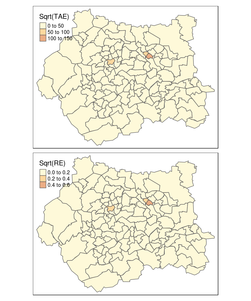
Figure 8.1: Geographical distribution of Total Absolute Error (TAE) and Relative Error (RE). Note the zones of high error are clustered in university areas such as near the University of Leeds, where there is a high non-resident population.
Note that the maps presented in Figure 8.1 look identical for TAE and RE values except for the scale; the similitude of these measures of fit can be verified using a simple correlation:
cor(TAEVec, REVec) # the measures are highly correlated## [1] 0.9963713In this case, both are quite well correlated. However, when having very different zones, in terms of total population, it can have more differences between the two maps. Indeed, with the same TAE, if the zone 84 had contained a total population two times bigger, the RE would be very smaller. Thus, RE would be divided by the multiplication of 2 and the number of variables.
Having identified a zone that is particularly problematic (the 84), we will look at the responsible variables. We focus on the zone 84 and calculate the number of differences between the constraint and the simulation for each category:
RudeDiff <- cons[84,] - ind_agg[84,] # differences for zone 84
diff <- round( abs(RudeDiff) ) # interesting differences

diff[diff > 1000] # printing the differences bigger than 1000
## m45_54 m55_64 Car NoCar
## 1274 1120 4960 4960The responsible variable seems to be the car ownership. We have made a similar check for the three worst zones and this variable is always the one with the largest difference. To investigate the reasons for this, we print the constraints for this variable inside the three worst zones and the marginals of the observed individuals:
worst <- tail(order(REVec), n = 3)
cons[worst, c("Car", "NoCar")] # constraint for 3 worst zones
## Car NoCar
## [1,] 6983 10927
## [2,] 11453 8040
## [3,] 8796 14204table( ind[,2] ) # individuals to weight (1 = Car ; 2= NoCar)##
## 1 2
## 738 178Only few observed individuals did not own a car. Thus, for zones needing a lot of persons that have no car, the weight of only 178 individuals out of 916 can be adapted. The possibility of having an individual that has the whole range of possible characteristics is then lower. The individuals without a car are saved in the NoCar variable. The contingency table of these people for the number of cakes and the age shows that we have nobody of age 55-64 eating more than 6 cakes.
# individuals not owning a car
NoCar <- ind[ind$Car==2,]

# Cross table
table(NoCar$NCakes,NoCar$ageband4)
##
## 16-24 25-34 35-44 45-54 55-64 65-74
## <1 3 5 3 5 4 6
## 1-2 10 11 8 5 5 5
## 3-5 9 13 6 10 3 8
## 6+ 7 10 3 4 0 10
## rarely 2 7 2 6 2 6The three zones with the worst simulation needed a lot of people without a car. On the contrary, below, we print the constraint of car of the three best zones. They needed less people of this category. This is the risk by generating a population of 1,623,800 of inhabitants and having a survey including only 916 persons.
best <- head(order(REVec), n = 3)
 # constraint for 3 best zones
cons[best, c("Car", "NoCar")]
## Car NoCar
## [1,] 12316 3705
## [2,] 8182 3952
## [3,] 10336 2597In conclusion, the simulation runs well for all zone excepts few ones. This is due to the individuals present in the sample. This could be explained by a survey that was not uniformly distributed through the different zones or does not include enough persons.
8.2 Empty cells
Roughly speaking, ‘empty cells’ refer to individuals who are absent from the input microdata. More specifically, empty cells represent individuals with a combination of attributes in the constraint variables that are likely to be present in the real spatial microdata but are known not to exist in the individual level data. Empty cells are easiest to envision when the ‘seed’ is represented as a contingency table. Imagine, for example, if the microdata from SimpleWorld contained no young males. The associated individual data could be Table 8.1, leading to the cross table shown in Table 8.2. We can clearly identify that there is no young male. Applying reweighting methods on this kind of input data result in an unrealistic final population, without young male.
| age | sex | |
|---|---|---|
| 1 | a50+ | m |
| 2 | a50+ | m |
| 4 | a50+ | f |
| 5 | a0_49 | f |
| f | m | |
|---|---|---|
| a0_49 | 1 | 0 |
| a50+ | 1 | 2 |
The importance of empty cells and methods for identifying whether or not they exist in the individual level is explained in a recent paper (Lovelace et al. (2015)). The number of different constraint variable permutations (\(Nperm\)) increases rapidly with the number of constraints (see equation below), where \(n.cons\) is the total number of constraints and \(n.cat_i\) is the number of categories within constraint \(i\):
\begin{equation} \displaystyle Nperm = \prod_{i = 1}^{n.cons} n.cat_{i} \label{eqempty} \end{equation}To exemplify this equation, the number of permutations of constraints in the SimpleWorld microdata example is 4: 2 categories in the sex variables multiplied by 2 categories in the age variable. Clearly, \(Nperm\) depends on how continuous variables are binned, the number of constraints and diversity within each constraint. Once we know the number of unique individuals (in terms of the constraint variables) in the survey (\(Nuniq\)), the test to check a dataset for empty cells is straightforward, based on equation :
\begin{equation} is.complete = \left\{ \begin{array}{ll} TRUE & \mbox{if } Nuniq = Nperm \\ FALSE & \mbox{if } Nuniq < Nperm \end{array} \right\} \end{equation}Once the presence of empty cells is determined, the next stage is to identify which types of individuals are missing from the individual level input dataset (\(Ind\)).
The `missing’ individuals, needed to be added to make \(Ind\) complete, can be defined by the following equation :
\[ Ind_{missing} = \{x | x \in complete \cap x \not \in Ind \} \]
This means simply that the missing cells are defined as individuals with constraint categories that are present in the complete dataset but absent from the input data.
8.3 External validation
Beyond mistakes in the code, more fundamental questions should be asked of results based on spatial microsimulation. The validity of the assumptions affect confidence one should have in the results. For this we need external datasets. External validation is therefore a tricky topic which is highly dependent on the available data (Edwards et al. 2010).
Geocoded survey data, real spatial microdata, is the ‘gold standard’ when it comes to official data. Small representative samples of the population for small areas can be used as a basis for individual level validation.
8.4 Chapter summary
This chapter explored methods for checking the results of spatial microsimulation, building on the CakeMap example presented in the previous chapter. This primarily involved checking that the results are internally consistent: that the output spatial microdata correspond with the geographical constraints. This process, generally referred to as ‘internal validation’, is important because it ensures that the model is internally consistent and contains no obvious errors.
However, the term ‘validation’ can be misleading as it implies that the model is in some way ‘valid’. A model is only as good as its underlying assumptions, which may involve some degree of subjectivity. We therefore advocate talking about this phase as ‘evaluation’ or simply ‘model checking’, if all we are doing is internal validation.
In the example of CakeMap, no datasets are available to check if the simulated rate of cake is comparable with that estimated from other sources. In the case of microsimulation, external validation is often difficult because available datasets are usually used for the simulation. This helps explain why internal validation is far more common in spatial microsimulation studies than external validation, although the latter is generally more important.
References
Chai, T., and R. R. RR Draxler. 2014. “Root mean square error (RMSE) or mean absolute error (MAE)? – Arguments against avoiding RMSE in the literature.” Geoscientific Model Development 7 (3): 1247–50. doi:10.5194/gmd-7-1247-2014.
Diez, David M, Christopher D Barr, and Mine Cetinkaya-Rundel. 2012. OpenIntro statistics. CreateSpace independent publishing platform.
Voas, David, and Paul Williamson. 2001. “Evaluating Goodness-of-Fit Measures for Synthetic Microdata.” Geographical and Environmental Modelling 5 (2). Routledge: 177–200. doi:10.1080/13615930120086078.
Lovelace, Robin, Dimitris Ballas, Mark M.H. Birkin, Eveline van Leeuwen, Dimitris Ballas, Eveline van Leeuwen, and Mark M.H. Birkin. 2015. “Evaluating the performance of Iterative Proportional Fitting for spatial microsimulation: new tests for an established technique.” Journal of Artificial Societies and Social Simulation 18 (2): 21.
Edwards, Kimberley L., Graham P. Clarke, James Thomas, and David Forman. 2010. “Internal and External Validation of Spatial Microsimulation Models: Small Area Estimates of Adult Obesity.” Applied Spatial Analysis and Policy 4 (4): 281–300. doi:10.1007/s12061-010-9056-2.
This seems to be because hiding or being ashamed of inevitable mistakes allows bad practice to continue unnoticed (Powell et al. 2011).↩
This is very intuitive, since by considering all constraint variables together, we have taken the whole population once for each variable.↩
Data frames will not work in this function and must be converted to matrices with
as.numeric.↩