11 The TRESIS approach to spatial microsimulation
This chapter, by Richard Ellison and David Hensher,36 presents an alternative approach to spatial microsimulation that involves both the generation and simulation of individuals in household units. The method, known as TRESIS, has been developed for many years at The University of Sydney. TRESIS is mature, well tested and has been designed at the Institute of Transport and Logistics Studies (ITLS) to help solve transport-related problems.
This is the first published implementation of one component of TRESIS in R. It does not use a package of its own (although the development of a TRESIS package implementing the TRESIS approach in R would be possible, building on the following code). Except for dplyr, stringr and mlogit (for data manipulation, string processing and multinomial logit models, respectively), the methods are written entirely in base R. Therefore, if you understand the R language well, this chapter can also be seen as a stand-alone introduction to the TRESIS method, from a technical standpoint.
The chapter is divided into four sections: an overview of the method with, reference to academic research (11.1); a demonstration of the generation of realistic households used in TRESIS, building on CakeMap input data (11.2); and an illustration of how demand models can be used to allocate these synthetic households to geographic zones (Section 11.3). The work concludes with a brief discussion of the merits of the approach and directions that one could develop the methods highlighted.
11.1 Overview of TRESIS modelling system
TRESIS is a Transport and Environment Strategy Impact Simulator originally developed by Professor David Hensher and others at the Institute of Transport and Logistics Studies (ITLS). TRESIS evolved from an earlier project for the Bureau of Transport and Communications Economics (Hensher 2002; Hensher and Ton 2002). The TRESIS software provides users with the ability to assess the impacts of a large number of transport and land-use policies on various systems linked to travel behaviour. These include the environment, user expenditure and government revenue. TRESIS incorporates an extensive model system including discrete and continuous choice models. These are combined with a process of population (or more accurately, household) synthesis and a set of equilibration criteria. TRESIS provides a powerful alternative to some more widely used microsimulation implementations for evaluating strategic projects (Hidas 2005).
Building on the practical focus of the book, the bulk of the substantive material focusses on the generation of synthetic households, which is described in detail. The methods and code blocks outlined below are not provided as ‘production ready’ methods but stepping stones towards further transport modelling work in R. Notwithstanding recent efforts such as the stplanr package,37 R is currently little-used in transport research, despite its power and flexibility. The chapter demonstrates how the synthetic populations generated through TRESIS can be used to identify where different types of households live using a residential location model. The chapter concludes with discussion of other important aspects of transport modelling that could be integrated into R, building on this work.
Overall, the TRESIS model system was designed to cover many of the long and short-term decisions made by individuals and households that affect how they travel. These range from the very long-term (e.g., where to live and where to work) to the very short-term (e.g., departure time and travel mode). When used together, the TRESIS models predict households’ long-term decisions and how these decisions then affect how individuals within that household travel given user-specified transport and land-use policies. Although in this chapter we discuss how to implement a stand-alone residential location model, the full power of the TRESIS system is only available when the whole set of demand models is estimated and run together. The figure below shows an overview of the high level TRESIS model structure (Hensher 2008).
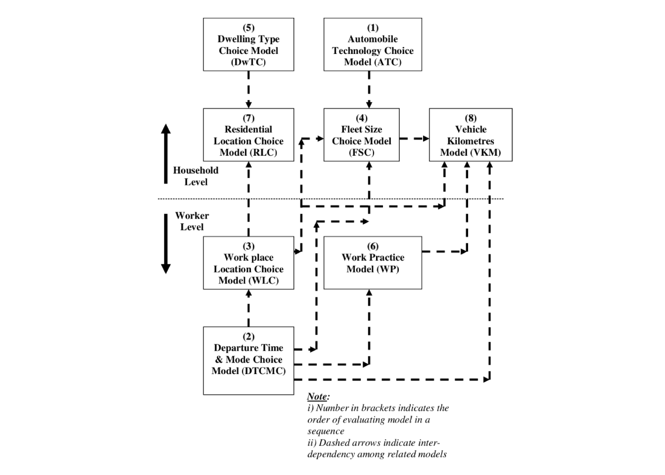
Figure 11.1: Overview of TRESIS model structure
The TRESIS demand models have been estimated from a combination of stated preference (SP) and revealed preference (RP) data using the NLOGIT software (see Hensher, Rose, and Greene (2015) for details of the software and estimation models). The model system provides for feedback between the different models using inclusive value parameters. These inclusive value parameters provide the mechanism through which the decisions made using one model (e.g., what vehicle to buy) are incorporated into the decisions made using other models in the system (e.g., where to live). In this chapter, we discuss only the stand-alone residential location model. This is just one part of TRESIS, which would be closely coupled to other sub-models covering fleet size, vehicle type choice, workplace location and dwelling type choice, among others (Hensher 2008).
11.1.1 Differences between TRESIS and other microsimulation systems
TRESIS differs from standard micro-simulation models in that it was designed primarily as a strategic model and in that it preserves the behavioural richness of observed individuals. In contrast, standard micro-simulation techniques commonly used in transport are largely designed for small-scale studies that cover only a small area and are typically focused on traffic simulation rather than behavioural simulation (Hidas 2005). TRESIS tends to operate at higher geographical levels than micro-simulation systems. Individuals in the household are not run through a micro-simulation model to determine specific routes. Instead, the TRESIS system estimates travel demand based on separate travel demand models within a network assignment model. Although this means that link level travel times for a specific individual cannot be determined, it provides more reliable aggregate estimates of travel time across the whole network. These are needed for the efficient running of the TRESIS models.
11.2 Synthetic households
11.2.1 What are synthetic households?
Synthetic households as used in TRESIS are a combination of a set of socio-demographic characteristics and a weight that represents their incidence in the population. These synthetic households form the building blocks for TRESIS and provide the necessary underlying variables required for the models in the simulation. The households are sampled such that given certain combinations of socio-demographic variables, there is a sufficiently large variation in the sample to reasonably cover all segments of the population that are of interest.
11.2.1.1 Synthetic households in TRESIS
There are fundamental differences between the populations generated through traditional population synthesis (described in earlier chapters) and synthetic households in TRESIS. First is that synthetic households retain their original composition and characteristics from the source sample. Rather than assigning sample individuals to households, in TRESIS individuals remain linked to their original households. Households are seen as a single entity, and used as the unit of analysis for many of the models, including the residential location model, within TRESIS. This has the side effect that each household is not simply a sum of its members but may also be considered to have its own characteristics.
Second is that synthetic households in TRESIS are not assigned to a unique geographic zone. Instead, the sample from which the synthetic households are drawn is limited to those households that are resident in the whole of the study area (generally a city’s Greater Metropolitan Area). This results in synthetic households having an overall geographic coverage matching the study area but no specific location within it. This approach means that the weights of the synthetic households are calculated based on their incidence in the entire population in the study area and not just their specific geographic location. The specific location of synthetic households is then assigned by running them through the TRESIS model and equilibrating the model system at trip, location and vehicle type levels. This reproduces with some accuracy the base year spatial travel and location profiles, as well as vehicle type and fleet size composition. Among others, TRESIS also includes a model for the choice of residential location using more disaggregate zones. It must be emphasised that household weights do not change when they are assigned to zones.
11.2.2 Required data for generating synthetic households
Like IPF and other population synthesis methods discussed previously, the generation of synthetic households in TRESIS requires a combination of micro level census data and aggregate population statistics.
The microdata needs to include matched household and individual level data. These are retained within the synthetic households. The aggregate population data should include the variables that are of most relevance to the research question for selecting synthetic households. The only requirement from the aggregate level data is that it includes a total count for the whole study area. The census data should ideally be available as a multi-way cross-tabulation for each combination of variables that are desired for representing the households in the target population. The reasons for this are explained further later in this chapter. For now suffice to say that the input data for TRESIS are all available from the census or other reliable sources in most advanced nations such as Australia, where the model was first developed for six of the state capital cities. The input data could come from different sources, however, if the variables are comparable.
11.2.3 Synthetic households in R
Generating synthetic households in R, using the TRESIS method, requires three stages. The first involves ensuring that the variables in the micro-data sample are compatible with those used in the demand models. Where variables used in the demand models or in the aggregate population level data are derived from one (or more) of the original micro-data variables, then these variables must be defined for each of the households in the micro-data sample. The second stage involves selecting variables on which to base the synthetic households and then calculating their weights and required sample. Third, the micro-data is sampled to generate the final synthetic households each with an individual weight based on their incidence in the population.
For this chapter, we will use the same CakeMap dataset as was used in the previous chapter. To ensure that we are using the base data without any modifications, re-import the CakeMap data files:
ind <- read.csv("data/CakeMap/ind.csv")
cons <- read.csv("data/CakeMap/cons.csv")
Recall that the CakeMap dataset records individuals and not households. This means we need to add a variable to the dataset that records which household each individual is in. Since we do not know who in the CakeMap dataset is in which household, for this example we will randomly assign each individual to a household:
set.seed(99) # This line sets the seed for the random number
# generation in the sample() function used below. This is
# used here to ensure that the results are consistent for each
# run. To ensure that your weighted of synthetic variables is
# reasonable for your application it is best to run this
# several times without a seed and compare the results.

# Randomly select the sizes of the households and then assign
# the unique IDs of each household to sequential individuals
# in the dataset.
ind$hhld <- rep(1:1000, times=sample(c(1:6), 1000, replace=TRUE)
                )[1:nrow(ind)]

# Check how many households we have in our dataset:
length(unique(ind$hhld))
## [1] 260Keep in mind that the sample() function randomly selects numbers so you will likely have a different number of households in your dataset unless you set the seed using set.seed(99) as above. Once we have assigned each individual to a dataset we can generate the household level data. For this example we can simply calculate some of these household variables including the number of individuals in the household, the number of workers and the age of the oldest person living in the household. Ensure you have loaded the dplyr and stringr packages and then run:
library(dplyr)
library(stringr)
hhlds <- group_by(ind, hhld) %>%
summarise(
numres = n(),
# Values of 8 and 97 mean "long-term unemployed" and
# "not answered" respectively
numworkers = length(NSSEC8[NSSEC8 < 8]),
nummanager = length(NSSEC8[NSSEC8 == 1.1]),
numprof = length(NSSEC8[NSSEC8 == 1.2]),
numrout = length(NSSEC8[NSSEC8 == 7]),
# Take the midpoint of the age ranges then take the maximum
# for that household
maxage = max(
rowMeans(
read.table(
text=str_replace(ageband4, '-', ','),
header=FALSE, sep=',')
)
),
# Value of 1 means they have a car, 2 means they do not.
# Divide the number of cars by 1.5 to get a more realistic
# number since more than 1 person can use the same car.
numcars = floor(sum((Car-2)*-1)/1.5)
)
hhlds[,c("hhld","numres","numworkers","nummanager",
"numprof","numrout","numcars")]## # A tibble: 260 x 7
## hhld numres numworkers nummanager numprof numrout numcars
## <int> <int> <int> <int> <int> <int> <dbl>
## 1 1 4 4 0 0 1 1
## 2 2 1 1 0 0 0 0
## 3 3 5 5 0 0 0 2
## 4 4 6 5 0 0 1 3
## 5 5 4 4 0 0 2 2
## 6 6 6 5 0 0 2 2
## 7 7 5 4 1 0 1 2
## 8 8 2 2 0 0 1 1
## 9 9 3 3 0 0 1 2
## 10 10 2 2 0 0 0 0
## # ... with 250 more rowsThis code uses dplyr’s group_by() and summarise() functions to generate the household level data from the individual level data. Generally, some household level data is already provided in the micro-data sample from the census but it may be necessary to add additional summary variables using the individual level micro-data.
The cons data frame from the CakeMap dataset contains the aggregate population level data we need for generating the weights and identifying the required sample. However, since the cons data frame is at the Ward level, we need to aggregate to get a total for all the wards. This is easy to accomplish by using the colSums() function:
totcons <- colSums(cons)Now that we have finished preparing the data, we can start generating the synthetic households. Just as with selecting the constraint variables in the previous chapter, we first need to choose which variables are the most important to ensure that our synthetic households reflect the distribution of these variables in the population. We should also select the number of households we want to generate. Which variables should be used depends on exactly what is being investigated. If it is of interest to identify how a specific policy will affect households with a different number of workers (e.g., peak hour congestion charging), then it is important to ensure that the number of workers is used as one of the variables in the generation of synthetic households. For this relatively simple dataset, we will use the availability of a car and the number of professionals in the household as the weighting and sampling variables. Typically, synthetic households in TRESIS are generated using three (nested) pairs of variables including household income, number of workers, family structure (e.g., family with children, family without children, single-person household, etc) and the occupation of the reference person, among others. However, since the cross-tabs are not available for the CakeMap data, for the purposes of this example we will assume that the distributions of the two variables (car and professionals) are the same for all combinations as they are for the population. Similarly, we will assume that the distribution for households is the same for individuals.38
First, let us look at the distributions of the two variables across the population using the prop.table() function:
# Car vs No Car:
prop.table(c(totcons['Car'],totcons['NoCar']))
## Car NoCar
## 0.701 0.299# Professionals vs All others:
prop.table(c(Professionals=totcons['X1.2'],
OtherOcc=sum(
totcons[c(match('X1.1', names(totcons)),
match('X2', names(totcons)):match(
'Other', names(totcons)
)
)])))## Professionals.X1.2 OtherOcc
## 0.0595 0.9405The prop.table() function takes two or more values and generates a table with the proportion of each value is of the total. The match() function is used to find the elements in the vector, names(totcons) containing the names of the variables in the totcons data frame, that match the relevant variable name. This is used here to avoid hard coding the correct index which we may change inadvertently. Using this code we see that approximately 30% of households in the population have no car and that only 6% of the population are professionals (occupation category 1.2). Given our assumption that these distributions also apply for all combinations, we can calculate that for the population as a whole using the tcrossprod() function:
popdistprop <- tcrossprod(
  prop.table(c(totcons['Car'],totcons['NoCar'])),
  prop.table(c(Professionals=totcons['X1.2'],
             OtherOcc=sum(
               totcons[c(
                 match('X1.1', names(totcons)),
                 match('X2', names(totcons)):match(
                   'Other', names(totcons)
                   )
               )])))
)
colnames(popdistprop) <- c('Professionals','Other')
rownames(popdistprop) <- c('Car','NoCar')
popdistprop
## Professionals Other
## Car 0.0417 0.659
## NoCar 0.0178 0.281This code uses the tcrossprod() function to take the two pairs of proportions we used earlier and multiplies all values in the first matrix by each value in the second. In this case this results in a 2x2 matrix that shows the distribution for the combination of the two variables. Keep in mind that this would not need to be a square matrix if the variables used have more than two values. From this we can calculate the actual number of households in each combination. Since the CakeMap dataset includes only the number of people rather than the number of households, we will need to make the assumption that each household has a certain number of people. If we assume that each household has an average of three people living there then we would use the code below to calculate the total number of households in each group in the population as a whole. Note that if you have the actual number of households in each group, this should be used instead.
popdisttot <- round(
    popdistprop*(totcons['Car']+totcons['NoCar'])/3
  )
popdisttot
## Professionals Other
## Car 22577 356923
## NoCar 9624 152143If we choose to generate 100 synthetic households, we simply need to multiply the matrix by 100 and then round to see how many households we need to sample from each of the for combinations of variables:
popdist <- round(popdistprop*100)
popdist
## Professionals Other
## Car 4 66
## NoCar 2 28In this case, each group has at least one household in the sample. However, when more variables are used (or variables with more values), it is common for several groups to be too small to have a sufficient proportion in the population to be represented in the synthetic households (particularly with only 100 households). When this occurs, these small groups are combined into a single larger group such that together they are represented by at least one household.
The last step before we sample the synthetic households is to generate the weights. Similar to other other methods of population synthesis discussed earlier in this book, the weights tell us how many real households each of our synthetic households represent in the population. This is calculated by simply dividing the total number of households in each group by the number in our set of synthetic households:
popweights <- popdisttot/popdistYou may choose to round the weights to ensure that each synthetic household represents only whole households but this is not absolutely necessary.
We can now sample the households with which to generate the synthetic households. Although it is possible to automate this process provided the variable names are mapped to each other, we will do this manually to illustrate the process. Taking the first group (professionals with a car) we can select the required number of households by using the following code:
synhhlds <- sample(
  filter(
    hhlds,numprof > 0, numcars > 0)$hhld,
  popdist['Car','Professionals']
  )
synhhldweights <- rep(
  popweights['Car','Professionals'],
  popdist['Car','Professionals']
  )
synhhldtypes <- rep(
  'Car+Professionals',
  popdist['Car','Professionals']
  )
The second line takes the calculated weights for that group of synthetic households and repeats it for the required number of households using the rep() function. The third line is used just to help identify from which group each household was sampled. This is generally not used but it can be useful for checking the results. Once we have sampled all the households we will bind the two vectors (synhhlds and synhhldweights) into a single data frame. Note that the use of the sample() function means that the specific households chosen will likely differ somewhat every time unless the set.seed() function is used first (as we did above). This is why it is important to select the correct variables because the only variables that are guaranteed to match the distribution in the population are those that are used to select the synthetic households. This is then repeated for each of the subsequent groups.39
This results in a vector with the household IDs of the households from the micro-data selected to be used for the synthetic households and a separate vector for the household weights. Since these two vectors are both in the same order, we can create a data frame that contains the synthetic household ID and the matching household weights.
synhhldDF <- data.frame(hhld=synhhlds,
                        hhldweight=synhhldweights,
                        hhldtype=synhhldtypes
                       )
Once this has been done generating the synthetic household dataset is relatively straightforward requiring us to merge the individual and household level data for our desired households. In TRESIS itself, this is followed by some additional work to ensure that any variables not required for the models are removed as well as making any necessary changes to ensure confidentiality of the micro-data is retained.
synhhlddata <- merge(
  filter(hhlds, hhld %in% synhhlds),
  filter(ind, hhld %in% synhhlds),
  by='hhld',
  all.x=TRUE,
  all.y=TRUE
)

# Merge with the weights data frame
synhhlddata <- merge(
  synhhlddata,
  synhhldDF,
  by='hhld',
  all.x=TRUE
)

# Add an ID for each individual in the household
# (starting from 1 for each household)
synhhlddata <- group_by(synhhlddata, hhld) %>%
  mutate(
    indid = 1:n()
  )
The synhhlddata data frame now contains all the data we need to use within the residential location model for assigning households to zones. So we can avoid regenerating synthetic households every time we change our residential location model, it is useful to save our data frame to an RData file:
save(synhhlddata,file="output/synhhlddata.RData")11.3 Using demand models to allocate synthetic households to zones using R
The key to the TRESIS system are its demand models. As discussed earlier in this chapter, the models used in TRESIS include a variety of discrete choice models covering many of the travel-related decisions made by individuals and households. The models used in TRESIS are linked meaning the model for residential location cannot be completely separated out from the rest of the models. However, the TRESIS approach can be used even with a single stand-alone residential location choice model and given its (potential) simplicity, it is this approach that will be discussed here.
At its most basic, a residential location model as used with the TRESIS synthetic households is a discrete choice model that predicts, up to a probability, in which area each household will choose to live given their unique set of socio-demographic characteristics and the characteristics of the different zones. Although the full details of the estimation of discrete choice models is outside the scope of this book, it is worth briefly discussing how the models used for TRESIS can be estimated. The discrete choice models used for residential location in TRESIS have been estimated from disaggregate choice data collected using a combination of revealed preference and stated preference surveys. It is also possible to estimate discrete choice models using micro level data provided sufficient spatial detail is available for your purposes. The models in TRESIS were estimated using the NLOGIT software package because it provides features needed for advanced models unavailable in most other packages. However, many discrete choice models as would be used by those developing residential location models can also be estimated in R using the mlogit and mnlogit packages.
11.3.1 Simple discrete choice model for residential location
The CakeMap data we are using does not have the disaggregate data we need to estimate the discrete choice model. For this reason, we will use a “model” where the parameters have been randomly selected. This means that our results in this case are unlikely to reflect the true values provided in the cons data frame. Nonetheless, the procedure we will use is the same as would be used if a properly estimated discrete choice model was available.
The discrete choice model that is needed is one where each alternative (zones in our study area) have an estimated utility function. The utility functions for each alternative can include either the same independent variables or different independent variables as well as common parameters or alternative-specific parameters. Since our dataset contains 124 wards, we will simplify our example by reducing these to 4 larger zones of 31 wards each. Zone 1 will include wards 1-31, zone 2 will include wards 32-62, etc. The model below was estimated based on using average values for each ward using a very simple model and cannot be regarded as a “good” model. However, it fits the required structure for the utility expressions and in the absence of disaggregate data for estimating the model we will use it for this example.
\[ \begin{aligned} U_1 &= \\ &3.3*mgmt + 1.85*rout + 1.73*numCars \\ U_2 &= \\ &6.56 - 1.35*prof + 26.81*mgmt - 0.83*rout - 3.11*numCars \\ U_3 &= \\ &0.12 - 1.08*prof + 1.4*mgmt + 1.78*rout + 1.99*numCars \\ U_4 &= \\ &3.71 - 8.09*prof + 33.24*mgmt + 1.81*rout - 1.29*numCars \end{aligned} \]
In this model, the subscript on U indicates the zone, mgmt is the number of workers in the household who are managers, prof is the number of workers who are professionals, rout is the number of workers whose occupation is considered “route”, and numCars is the number of cars in the household.
Applying the model requires the values of each of the synthetic households to be run through the utility equations to calculate the probabilities of the households living in each of the four zones. The easiest way to calculate the utilities for each synthetic household is to make use of R’s vector functionality. Since our model includes only household level characteristics, we begin by simplifying the synthetic household data to one row per household with only the variables necessary for our model, making sure to rename them to match the variable names in our utility expressions:
synrun <- unique(synhhlddata[,c("hhld","nummanager","numprof",
                                "numcars","numrout",
                                "hhldweight","hhldtype")])
synrun <- rename(synrun,
                 mgmt = nummanager,
                 prof = numprof,
                 numCars = numcars,
                 rout = numrout
                 )
We then create variables for each of the four utility expressions. The while loop iterates through each of the utility expressions to calculate the relevant utilities.40 The eval() and parse() functions are used together to take text input and evaluate the expressions as if R code had been typed into the console or a standard R script file. The with() function allows the variable names in the utility expressions to be used as-is, without pre-pending the data frame name and a $ to them and not attaching the data frame to the global environment.
synrun <- synrun %>% mutate(
  u1 = NA,
  u2 = NA,
  u3 = NA,
  u4 = NA
)
i <- 1;
while (i <= 4) {
  synrun[,7+i] <- with(synrun,
       eval(parse(text=c(
         "3.2989*mgmt + 1.8519*rout +
         1.733*numCars",
         "6.5633 - 1.3535*prof + 26.8106*mgmt - 0.8307*rout -
         3.1094*numCars",
         "0.115 - 1.0771*prof + 1.3984*mgmt + 1.781*rout +
         1.9871*numCars",
         "3.7052 - 8.0874*prof + 33.2434*mgmt + 1.8073*rout -
         1.291*numCars"
       )[i])))
  i <- i + 1
}
We can then calculate the probabilities of each synthetic household living in each zone. The equation to estimate the probabilities depend on the exact model specification that is used in the model. In this case, where the model includes alternative-specific variables (and values), we can use the equations below. These probabilities can then be used to help identify where households sharing the characteristics of each synthetic household are likely to live:
synrun <- synrun %>% mutate(
  p1 = exp(u1)/(exp(u1)+exp(u2)+exp(u3)+exp(u4)),
  p2 = exp(u2)/(exp(u1)+exp(u2)+exp(u3)+exp(u4)),
  p3 = exp(u3)/(exp(u1)+exp(u2)+exp(u3)+exp(u4)),
  p4 = exp(u4)/(exp(u1)+exp(u2)+exp(u3)+exp(u4))
)
The final probabilities for 10 households are shown in the table below. In this very simple example, you will see that there are some households with the same probabilities. Given a fully developed residential location model as the one used in TRESIS, with more explanatory variables as well as a wider range of grouping variables for the synthetic households, the number of households with the same probabilities would be very low. However, even from this relatively simplistic example, it is apparent that even within the same groups, the probabilities of living in a particular zone vary (sometimes substantially).
| hhld | hhldweight | hhldtype | p1 | p2 | p3 | p4 |
|---|---|---|---|---|---|---|
| 1 | 5408 | Car+Other | 0.22 | 0.08 | 0.29 | 0.41 |
| 4 | 5408 | Car+Other | 0.31 | 0.00 | 0.69 | 0.00 |
| 5 | 5408 | Car+Other | 0.37 | 0.00 | 0.60 | 0.03 |
| 6 | 5408 | Car+Other | 0.37 | 0.00 | 0.60 | 0.03 |
| 7 | 5408 | Car+Other | 0.00 | 0.00 | 0.00 | 1.00 |
| 10 | 5434 | NoCar+Other | 0.00 | 0.94 | 0.00 | 0.05 |
| 13 | 5408 | Car+Other | 0.10 | 0.56 | 0.14 | 0.20 |
| 16 | 5408 | Car+Other | 0.22 | 0.08 | 0.29 | 0.41 |
| 18 | 5434 | NoCar+Other | 0.00 | 0.94 | 0.00 | 0.05 |
| 20 | 5408 | Car+Other | 0.22 | 0.08 | 0.29 | 0.41 |
11.3.2 Results
The final step is to assign the number of households in each zone using the probabilities and the household weights. Although in some applications the highest probability is assumed to be the chosen zone, in the TRESIS approach, the probabilities are used in combination with the weights to identify how many real households with the same characteristics as the synthetic households would live in each zone.
synresults <- synrun %>%
  group_by(hhldtype) %>%
  summarise(
    zone1 = round(sum(p1*hhldweight)),
    zone2 = round(sum(p2*hhldweight)),
    zone3 = round(sum(p3*hhldweight)),
    zone4 = round(sum(p4*hhldweight))
  )
The results of this (very basic) model are shown in the table below. These initial results do not accurately reflect the shares in the population in each zone. This is for a number of reasons. The primary reason is that the example model we used here was by many measures a poor model with very low goodness of fit, including a very low \(R^2\) value and a highly insignificant \(\chi^2\) p-value. If a better model had been estimated using disaggregate data, the results would be much closer to the actual population shares.
| hhldtype | zone1 | zone2 | zone3 | zone4 |
|---|---|---|---|---|
| Car+Other | 77737 | 38230 | 137451 | 103505 |
| Car+Professionals | 12075 | 3172 | 7327 | 3 |
| NoCar+Other | 524 | 130409 | 560 | 20651 |
| NoCar+Professionals | 52 | 9551 | 20 | 1 |
The second reason for the difference is that the model we used was not calibrated on the population shares. The TRESIS models are calibrated to ensure they reproduce the shares in the base period before being used to run any analysis. Calibration is not a straightforward process but involves adjusting the alternative-specific constants in the model until the estimated shares match the population shares within an acceptable level of tolerance.
Although we will not run the calibration procedure here, to illustrate the sensitivity of the results to the quality of the model and the need for calibration, we will re-run the calculations with small changes to the alternative-specific constants of the utility expressions. If we decrease the value of the alternative-specific constant of zone 2 so that the utility expressions become:
\[ \begin{aligned} U_1 &= \\ &3.299*mgmt + 1.852*rout + 1.73*numCars \\ U_2 &= \\ &5.56 - 1.35*prof + 26.8*mgmt - 0.830*rout - 3.11*numCars \\ U_3 &= \\ &0.115 - 1.08*prof + 1.40*mgmt + 1.78*rout + 1.99*numCars \\ U_4 &= \\ &3.705 - 8.09*prof + 33.2*mgmt + 1.81*rout - 1.29*numCars \end{aligned} \]
| hhldtype | zone1 | zone2 | zone3 | zone4 |
|---|---|---|---|---|
| Car+Other | 81765 | 20811 | 143302 | 111045 |
| Car+Professionals | 13107 | 1633 | 7833 | 4 |
| NoCar+Other | 949 | 112580 | 1022 | 37592 |
| NoCar+Professionals | 140 | 9429 | 53 | 2 |
Decreasing the constant for zone 2 further results in more changes. It is important to understand that the probabilities do not change linearly in response to an equal change in the value of the alternative-specific constant. Furthermore, the switch between zones is not equal across the groups. As a result, calibration involves the incremental changes of more than one alternative-specific constant until the shares are reproduced.
\[ \begin{aligned} U_1 &= \\ &3.30*mgmt + 1.85*rout + 1.73*numCars \\ U_2 &= \\ &4.56 - 1.35*prof + 26.8*mgmt - 0.830*rout - 3.11*numCars \\ U_3 &= \\ &0.115 - 1.078*prof + 1.40*mgmt + 1.78*rout + 1.99*numCars \\ U_4 &= \\ &3.71 - 8.09*prof + 33.2*mgmt + 1.81*rout - 1.29*numCars \end{aligned} \]
| hhldtype | zone1 | zone2 | zone3 | zone4 |
|---|---|---|---|---|
| Car+Other | 84377 | 9412 | 147087 | 116048 |
| Car+Professionals | 13726 | 710 | 8137 | 4 |
| NoCar+Other | 1549 | 87167 | 1685 | 61743 |
| NoCar+Professionals | 368 | 9111 | 141 | 5 |
11.4 Conclusions
This chapter has described the process required for generating and applying the synthetic households used within the TRESIS model system to a more general application of population synthesis. Although TRESIS is a land-use and transport simulator, the approach described here is a generalised one that is applicable to a wide range of model systems that require, or would benefit from, the use of disaggregate data for simulating decision making involving spatial decisions including residential location but also workplace location and other activity destinations.
11.4.1 Limitations
The primary limitation of the TRESIS approach to population synthesis is its heavy reliance on detailed disaggregate household and population level data. This means that acquiring the necessary data needed for generating the synthetic households and estimating and calibrating the models is frequently a time-consuming and sometimes expensive undertaking. In many contexts such data simply does not exist.
However, once the data has been collected, the resulting model system is very powerful, allowing predictions not only of the current state, but also of future forecasts of decisions under uncertainty. Provided the variables on which the forecasts rely are available in the synthetic households and models and are trustworthy, the TRESIS approach provides an integrated framework for modelling transport decisions.
11.4.1.1 Freight models
TRESIS has until recently been focused entirely on passenger transport with freight transport considered as part of the capacity of the network but not considered in the demand models. As such, the methods developed for TRESIS have been optimised for passenger transport modes. However, there is ongoing development within the Institute of Transport and Logistics Studies to develop freight and light commercial vehicle models. These models, although different in some ways to the passenger models, have been found fit in well with the concept of synthetic households. In contrast to the passenger models that rely on synthetic households, the freight and commercial vehicle models have applied the concept used for generating synthetic households, to firms resulting in the development of “synthetic firms”. Just as synthetic households are a collection of socio-demographic variables, synthetic firms are a collection of firm level (and worker) characteristics. The data requirements of synthetic households are however also problematic for synthetic firms.
11.4.2 MetroScan-TI
TRESIS, although extremely powerful in many ways, has lacked some features that are increasingly being needed for a full assessment of potential transport and infrastructure projects. MetroScan-TI is the latest evolution of the TRESIS model system that is currently being developed and incorporates all the behavioural richness of the original TRESIS models and extends this to include a much more detailed zone structure, a fully integrated network assignment model, freight models, models for firm location and modules for cost-benefit analysis and wider economy impact assessments. MetroScan-TI is intended to provide users with the ability to quickly and easily prioritise a large number of potential projects on a wide range of variables. These projects include the standard transport infrastructure (new railway lines, roads and service improvements) as well as other infrastructure and strategic level property development (the mix and number of flats, semi-detached and detached houses).
11.4.3 Extending residential location to transport models in R
Residential location models are an important component of any fully integrated transport model because they provide the “productions” (i.e., demand) for travel. However, at a minimum transport models also require a method of estimating the likely destinations (or “attractions”) of trips, as well as the mode used for these trips. The TRESIS approach uses the same synthetic households, and the individuals within those households, as were used in this chapter for the residential location model, to estimate the destinations and modes of trips. This means the development of a full transport model in R can apply the synthetic household method described in this chapter. Although developing the full set of models cannot be described as a simple process, as demonstrated in this chapter, the functionality of R, and some of its packages, makes it well suited to applying transport models. In particular, implementing full network assignment in R is likely to be particularly challenging, but its data structures and rapidly improving GIS functionality, some of which has been demonstrated in this chapter, means these are also likely to be possible.
11.5 Chapter summary
This chapter has provided an introduction to the TRESIS approach to population synthesis through the use of synthetic households and demand models. In it we learned to generate, allocate and model household level data. TRESIS is an approach that is relatively simply conceptually but that incorporates powerful behavioural features. This, combined with its ability to model a wide range of phenomena and behaviours in the synthetic households, makes TRESIS well suited to implementation in R (subject to data requirements). It can also be applied to a variety of other applications not limited to those involving transport models.
References
Hensher, David A. 2002. “A Systematic Assessment of the Environmental Impacts of Transport Policy.” Environmental and Resource Economics 22 (1). Springer: 185–217. http://www.springerlink.com/index/FJHH830P34VQBANM.pdf.
Hensher, David A, and Tu Ton. 2002. “TRESIS: A transportation, land use and environmental strategy impact simulator for urban areas.” Transportation 29 (4). Springer: 439–57.
Hidas, Peter. 2005. “A functional evaluation of the AIMSUN, PARAMICS and VISSIM microsimulation models.” Road & Transport Research 14 (4): 45–59.
Hensher, David A. 2008. “Climate change, enhanced greenhouse gas emissions and passenger transport - What can we do to make a difference?” Transportation Research Part D: Transport and Environment 13 (2): 95–111. doi:10.1016/j.trd.2007.12.003.
Hensher, David A, John M Rose, and William H Greene. 2015. Applied Choice Analysis. Second Edi. Cambridge: Cambridge University Press.
Richard B. Ellison and David A. Hensher are based at Institute of Transport and Logistics Studies, The University of Sydney Business School, The University of Sydney.↩
See https://github.com/ropensci/stplanr for more information.↩
This will generally not be the case in reality and so every effort should be made to source multi-way cross tab data for the required variables.↩
The code for this stage is over 50 lines long so is not included in the book. See the online version of the chapter of http://git.io/vGAEz for the code.↩
It is possible to extract the coefficients and variables names directly from the output of mlogit if desired. The text format is shown here since models estimated using nlogit are generally written in this format.↩