2 SimpleWorld: A worked example of spatial microsimulation
This chapter focuses on the minimum input datasets needed for the classical type of microsimulation. We will use input data on the inhabitants of an imaginary world (geographical individual level) called SimpleWorld to demonstrate the basic concepts and techniques to perform spatial microsimulation with R.
This is the first practical chapter and it aims to acquaint you with language R and the R development program RStudio. Fluency with R and RStudio, in combination with well-organised project management and clear, commented code, will enable fast and efficient work. In short, this chapter aims to teach good ‘workflow’ in preparation for navigating the subsequent chapters. A secondary aim is to illustrate key concepts in spatial microsimulation with reference to a practical example, called ‘SimpleWorld’ for its simplicity.
The chapter also serves to highlight the links between the methodology presented in-depth later in the book (see Chapter 5) and the various real-world applications presented in Chapter 4. For R ‘newbies’ it also provides a chance for the reader to do some basic programming in R: the unwritten subtitle of this book is “a practical introduction” for a reason!
This chapter is ordered as follows:
- Getting setup with the RStudio environment (2.1) contains the basic explanation of RStudio to enable you to code the examples of this book on your own computer.
- SimpleWorld data (2.2) describes the context and the data of this little illustrative example.
- Generating a weight matrix (2.3) contains the code and the description of the role of a weight matrix in a spatial microsimulation. -Spatial microdata (2.4) shows the typically useful output of a spatial microsimulation. -SimpleWorld in context (2.5) mentions the kind of context where the output could be used.
2.1 Getting setup with the RStudio environment
Before progressing further, it is important to ensure that R is setup correctly and working on your computer, so you can follow the practical examples. This section will not go into much detail. Further resources are provided in the Appendix at the end of the book to provide insight into how R works as a programming language.
The majority of the help that you need to install and setup R on your computer can be found online, so it is recommended that you consult this section with reference to online searches and help pages. As with all open source software projects R evolves over time so it is important to keep up-to-date with any changes, which may not be accounted for in this book.
2.1.1 Installing R
The practical examples in this book require a recent version of R to be installed on your computer. This will allow you to type test the code as you learn the methods. To install R, we recommend you refer to documentation provided online, on the Comprehensive R Archive Network (CRAN):
- For Windows, see https://cran.r-project.org/bin/windows/base/
- For Mac, see https://cran.r-project.org/bin/macosx/
- For Linux, see https://cran.r-project.org/doc/manuals/r-release/R-admin.html
On Debian-based systems such as Ubuntu, the following bash command should be sufficient to install R.
sudo apt-get install r-baseOnce R is installed, new packages are easy to install from within R using install.packages("package_name"). To install the mipfp package, for example, we would use:
install.packages("mipfp")2.1.2 RStudio
RStudio is an Integrated Development Environment (IDE) for R. It provides an advance Graphical User Interface (GUI) that makes it easier not only to write R code, but to install packages, manage R’s graphical outputs and organise complex projects. All R code presented in this book will run in other environments, such as Linux’s bash shell, in which R can be initiated by the following command:
$ R # enter the R command lineIt is highly recommended that you use RStudio for the work presented in this book, however, especially if you an R beginner. RStudio will enable you to spend less time worrying about how to write R code correctly and more time focussed on spatial microsimulation. One example of how RStudio saves time is its tab autocompletion functionality. To test this functionality, type the beginning of any R object or function stored in R’s environment (such as plo, short for plot) and hit the Tab button. The full name of various options should auto-complete, as illustrated in Figure 2.1. Pressing the down arrow allows the user to select the correct input. Auto-completion allows fast typing, easy recollection of function/object names. It also prevents errors cause by typos in your code.
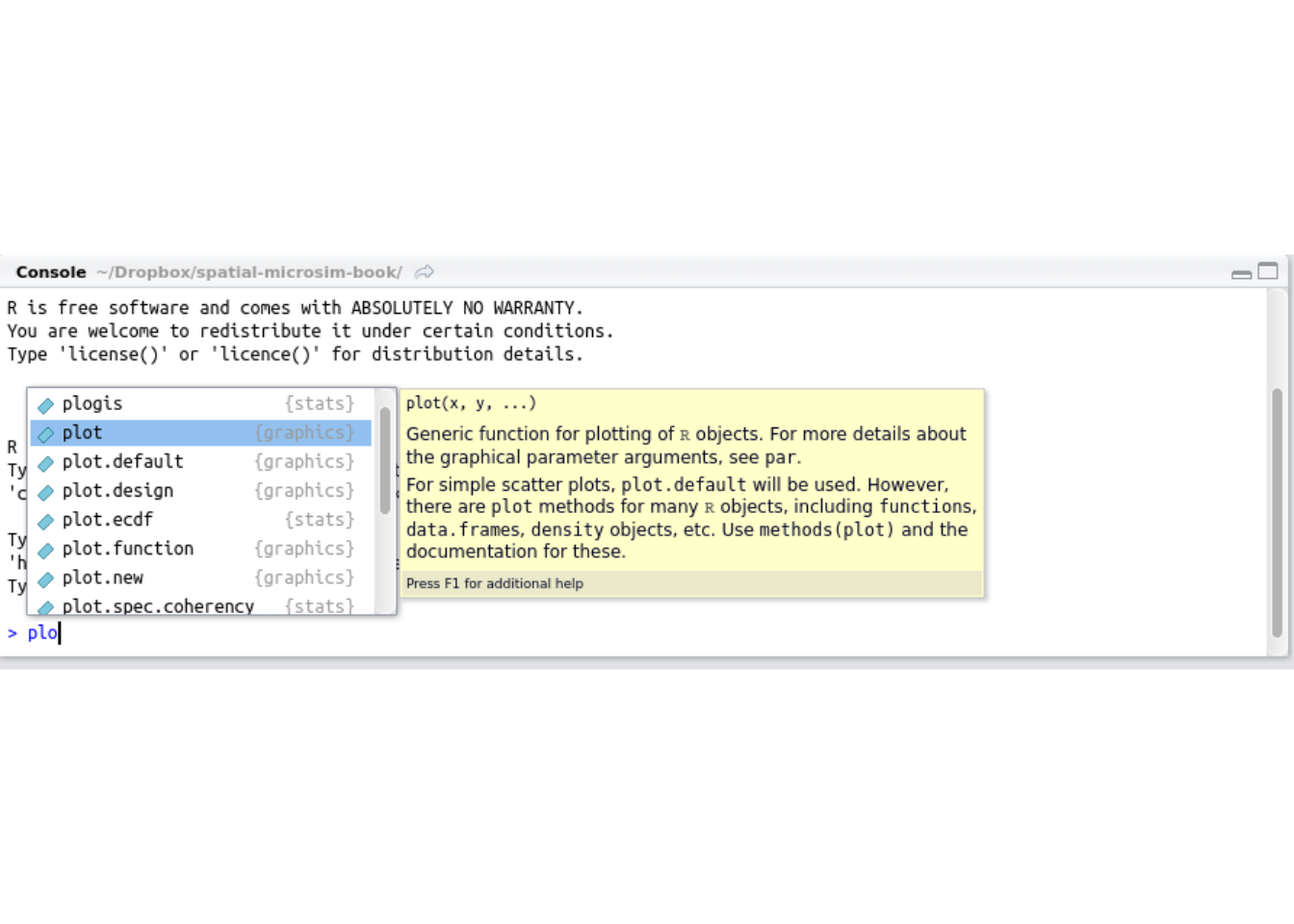
Figure 2.1: Autocompletion in RStudio
To test this functionality, download and install RStudio if you have not already. The installation process is simple on Linux, Mac and Windows platforms: simply follow the instructions provided here at rstudio.com/products/rstudio/download/.
There are many other advantages of using RStudio.5 The next section focuses on one particular advantage that we recommend you make use of whilst working through the book: RStudio projects.
2.1.3 Projects
RStudio provides a neat system for creating, managing and even sharing your projects. This functionality merits a section of its own, because spatial microsimulation projects are likely to be large and complex, requiring collaboration with other people. If you are not careful the projects can become over-complex and unmanageable. RStudio projects can prevent this from happening and lead to improved workflow.
To setup a new project click on the drop-down menu in the top-right section of RStudio. If you are working on a project, the name of the project will appear in this dropdown menu (see Figure 2.2). When a project is loaded, the following things happen:
- The files open in the script panel (top left) last time you worked on the project will appear.
- R’s working directory (set and checked with
setwd()andgetwd(), respectively) will change. - Any R objects saved in the
.RDatafile in the project will be automatically loaded, saving your work. - If you are using
gitto manage your project’s development and sharing, you’ll have options to commit code and ‘push’ new work, e.g. to GitHub.
In fact, this entire book was written as an RStudio project. This allowed us to work from the same system and share code easily, by pushing our code frequently to the book’s online repository: https://github.com/Robinlovelace/spatial-microsim-book . This online repository will allow you to access all of the example code and data for the book. It will also allow you to contribute to the book as an evolving project.
The next section explains how to download and use the data stored in the spatial-microsim-book GitHub repository to access the code and data resources associated with the book.
2.1.4 Downloading data for the book
To simply download the code and data, associated with this book, first navigate to https://github.com/Robinlovelace/spatial-microsim-book in your browser. From this page, click on the ‘Download ZIP’ button to the right and extract the folder into a sensible place on your computer, such as the Desktop.6
With the files safely stored on the computer, the next step is to open the folder as an RStudio project. To do this, open the folder in a file browser and double click on spatial-microsim-book.Rproj. Alternatively, start RStudio and open the file by clicking on ‘Open Project’ from the dropdown menu above the top-right panel, or by clicking with File > Open. This will cause RStudio to open the project. All the input data files should now be easily accessible to R through relative file paths. The files should also be visible in the Files tab in bottom right panel.
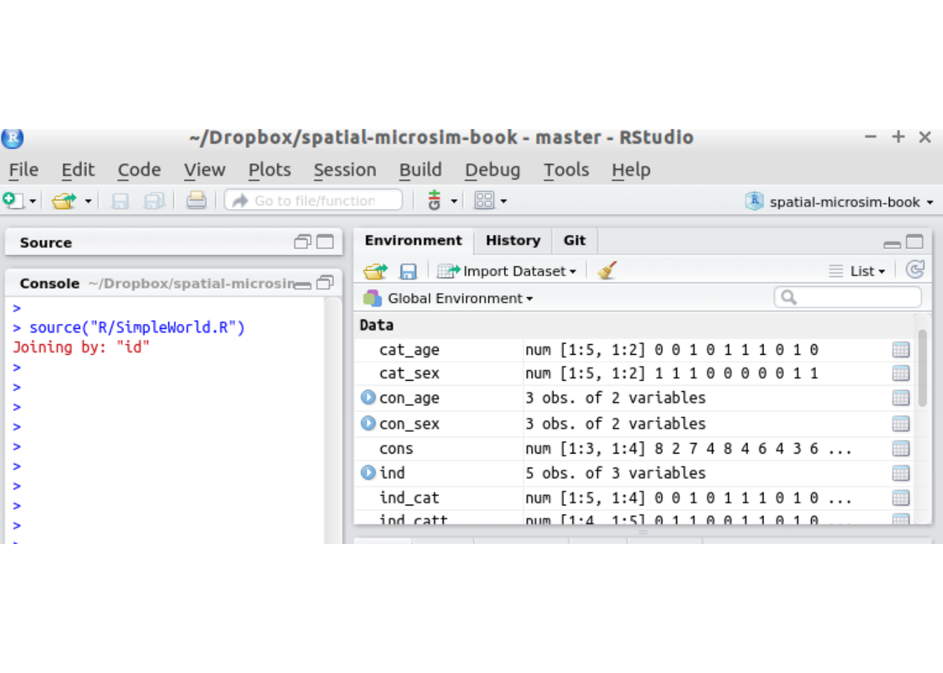
Figure 2.2: The RStudio interface with the spatial-microsim-book project loaded and objects loaded in the Environment after running SimpleWorld.R
To check if the project has been downloaded and opened correctly, try running the following code, by typing it and hitting Ctl-Enter:
source("code/SimpleWorld.R")You should see some output in red, beginning Attaching package: ‘dplyr’. Some new objects should also appear in the Environment tab in the top-right panel (Figure 2.2). This is the result of running the code located in a script file called SimpleWorld.R, using the source() function.
Now that you have an understanding of RStudio and how to load the book project, it’s time to ‘get your hands dirty’ and run some code! In the subsequent section we will type and run some of the contents of the SimpleWorld.R script line by line.
2.2 SimpleWorld data
SimpleWorld is a small world, consisting of 33 persons split across 3 zones, as illustrated in Figure 2.3. We have two sources of information about these people available to us:
- aggregate counts of persons by age and sex in each zone (from the SimpleWorld Census)
- survey microdata recording more detailed information (age, sex and income), for five of the world’s residents.
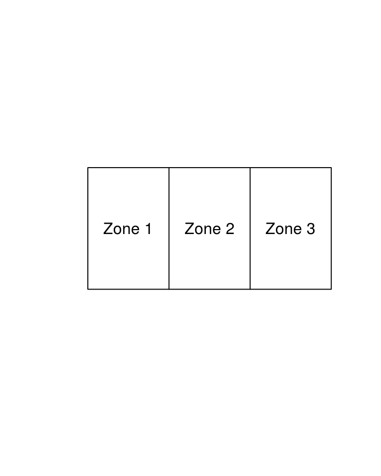
Figure 2.3: The SimpleWorld environment, consisting of individuals living in 3 zones.
Unfortunately the survey data lack geographical information, and include only a small subset of the population (5 out of 33). To infer further information about SimpleWorld — and more importantly to be able to model its inhabitants — we need a methodology. This is precisely the kind of situation where spatial microsimulation is useful. After an explanation of this ‘starting simple’ approach, we describe the input data in detail, demonstrate what spatial microdata look like and, finally, place the example in its wider context.
This SimpleWorld example is analogous to the ‘cartoon world’ used by professor MacKay (2008) to simplify the complexities of sustainable energy. The same principle works here: we will generate a synthetic population for the imaginary SimpleWorld to illustrate how spatial microsimulation works and how it can be useful.
The SimpleWorld planet, a 2 dimensional plane split into 3 zones, is illustrated in Figure 2.3. SimpleWorld is inhabited by 12, 10 and 11 individuals of its alien inhabitants in zones 1 to 3, respectively: a planetary population of 33. From the SimpleWorld Census, we know how many young (strictly under 50 space years old) and old (50 and over) residents live in each zone, as well their genders: male and female. This information is displayed in the tables below.
| zone | 0-49 yrs | 50 + yrs |
|---|---|---|
| 1 | 8 | 4 |
| 2 | 2 | 8 |
| 3 | 7 | 4 |
| Zone | m | f |
|---|---|---|
| 1 | 6 | 6 |
| 2 | 4 | 6 |
| 3 | 3 | 8 |
The following commands load-in this data.
# Load the constraint data
con_age <- read.csv("data/SimpleWorld/age.csv")
con_sex <- read.csv("data/SimpleWorld/sex.csv")
cons <- cbind(con_age, con_sex)
We recommend R beginners interact with the R objects just loaded: try printing them to screen, plotting them and even-subsetting them. If you cannot, it may be worth consulting the Appendix on using R, or referring to R’s copious online documentation. The data contained in the cons object presented below refer to the characteristics of inhabitants in different SimpleWorld zones.
cons # print the constraint data to screen## a0.49 a.50. m f
## 1 8 4 6 6
## 2 2 8 4 6
## 3 7 4 3 8Each row represents a new zone (see also Tables 2.1 and 2.1). The planet’s entire population is represented in the counts in these tables. From these constraint tables we know the marginal distributions of the two categorical variables, age and sex. The data does not tell us about the contingency table (or cross-tabulation) that links age and sex. This means that we have per-zone information on the number of young and old people and the number of males and females. But we currently lack information about the number of young females, young males, and so on. Also note that we have no information about other important variables such as income.
Spatial microsimulation can be used to better understand the population of SimpleWorld. To do this, we need some additional information: an individual level microdataset.
This is provided in an individuals level dataset on 5 of SimpleWorld’s inhabitants (Table 2.3). Note that the individual level data has different dimensions than the aggregate data presented above.
| id | age | sex | income |
|---|---|---|---|
| 1 | 59 | m | 2868 |
| 2 | 54 | m | 2474 |
| 3 | 35 | m | 2231 |
| 4 | 73 | f | 3152 |
| 5 | 49 | f | 2473 |
The individual level microdata survey has one row per individual whereas the constraints have one row per zone. This individual level data includes two variables that link it to the aggregate level data described above: age and sex. The individual level data also provides information about a target variable not included in the geographical constraints: income. To load the individual level data, enter the following:
ind <- read.csv("data/SimpleWorld/ind-full.csv")Note that although the microdataset contains additional information about the inhabitants of SimpleWorld, it lacks geographical information about where each inhabitant lives or even which zone they are from. This is typical of individual level survey data. Spatial microsimulation tackles this issue by allocating individuals from a non-geographical dataset to geographical zones in another.
2.3 Generating a weight matrix
The process to generate spatial microdata is allocating weights to each individual for each zone. The higher the weight for a particular individual-zone combination, the more representative the individual is of that zone. This information can be represented as a weight matrix.
The subsequent code block uses the mipfp package to convert these inputs into a matrix of weights. Just type it in and observe the result. If it works, congratulations! You have generated your first weight matrix using Iterative Proportional Fitting (IPF) (see code output). The details of this process are described in subsequent chapters.
target <- list(as.matrix(con_age[1,]), as.matrix(con_sex[1,]))
descript <- list(1, 2)
ind$age_cat <- cut(ind$age, breaks = c(0, 50, 100))
seed <- table(ind[c("age_cat", "sex")])

library(mipfp) # install.packages("mipfp") is a prerequisite
res <- Ipfp(seed, descript, target)
res$x.hat # the result for the first zone
## sex
## age_cat f m
## (0,50] 4.455996 3.544004
## (50,100] 1.544004 2.455996Note that the output of the above command is only for the first zone. It suggests that in zone 1, younger females are far more (nearly 4.5 times more) numerous than would be expected based on the individual level data alone. This makes sense because con_age[1,] contains many young people and ind contains only one young female. At this stage you may be wondering: what just happened? This is explained in detail in the subsequent chapters.
An alternative approach to arriving at a similar result, for all zones, is demonstrated in the code chunk below using another package: ipfp. The result of this code is illustated in Table 2.4. Again, the reader is not expected to understand what has just happened. This will be explained in subsequent chapters.
A <- t(cbind(model.matrix(~ ind$age_cat - 1),
           model.matrix(~ ind$sex - 1)[, c(2, 1)]))

cons <- apply(cons, 2, as.numeric) # convert to numeric data

library(ipfp) # install.packages("ipfp") is a prerequisite
weights <- apply(cons, 1, function(x) ipfp(x, A, x0 = rep(1, 5)))
weights[,1] # result for the first zone
## [1] 1.227998 1.227998 3.544004 1.544004 4.455996| Individual | Zone 1 | Zone 2 | Zone 3 |
|---|---|---|---|
| 1 | 1.23 | 1.73 | 0.725 |
| 2 | 1.23 | 1.73 | 0.725 |
| 3 | 3.54 | 0.55 | 1.550 |
| 4 | 1.54 | 4.55 | 2.550 |
| 5 | 4.46 | 1.45 | 5.450 |
The highest value (5.450) is located, to use R’s notation, in cell weights[5,3], the 5th row and 3rd column in the matrix weights. This means that individual number 5 is considered to be highly representative of Zone 3, given the input data in SimpleWorld. This makes sense because there are many (7) young people and many (8) females in Zone 3, relative to the input microdataset (which contains only 1 young female). The lowest value (0.55) is found in cell [3,2]. Again this makes sense: individual 3 from the microdataset is a young male yet there are only 2 young people and 4 males in zone 2. A special feature of the weight matrix above is that each of the column sums is equal to the total population in each zone.
Note that the first method gives weights to categories (for example young female), whereas the second method gives weights to each individual. This is normal and equivalent, we can easily transform one type of output in the other type. The details are explained further.
We will discover different ways of generating such weight matrices in subsequent chapters. For now it is sufficient to know that the matrices link individual level data to geographically aggregated data and that there are multiple techniques to generate them. The techniques are sometimes referred to as reweighting algorithms in the literature (Tanton et al. 2011). These include deterministic methods such as Iterative Proportional Fitting (IPF) and probabilistic methods that rely on a pseudo-random number generator such as simulated annealing (SA). These and other reweighting algorithms are described in detail in Chapter 5.
2.4 Spatial microdata
A useful output from spatial microsimulation is what we refer to as spatial microdata. This is a dataset that contains a single row per individual (as with the input microdata) but also an additional variable on geographical location.
The ideal spatial microdataset selects individuals representative of the aggregate constraints for each zone, while containing the diversity of information present in the individual level non-spatial input population. In Chapter 4 we will explore all the steps needed to produce a spatial microdataset for SimpleWorld. A subset of such spatial microdataset is presented in Table 2.5, where each row represents an individual taken from the individual level sample and the ‘zone’ column represents the geographical zone in which they reside.
| id | zone | age | sex | income |
|---|---|---|---|---|
| 1 | 2 | 59 | m | 2868 |
| 2 | 2 | 54 | m | 2474 |
| 4 | 2 | 73 | f | 3152 |
| 4 | 2 | 73 | f | 3152 |
| 4 | 2 | 73 | f | 3152 |
| 4 | 2 | 73 | f | 3152 |
| 5 | 2 | 49 | f | 2473 |
| 4 | 2 | 73 | f | 3152 |
| 5 | 2 | 49 | f | 2473 |
| 2 | 2 | 54 | m | 2474 |
Table 2.5 is a reasonable approximation of the inhabitants of zone 2: older females dominate in both the aggregate (which contains 8 older people and 6 females) and the simulated spatial microdata (which contains 8 older people and 6 females). Note that in addition to the constraint variables, we also have an estimate of the income distribution in SimpleWorld’s second zone.
By the end of Chapter 5, you should learn how to generate this table and understand each of the steps involved. The remainder of this section considers how the outputs of spatial microsimulation, in the context of SimpleWorld, can be useful before progressing to the practicalities.
2.5 SimpleWorld in context
Even though the datasets are tiny in SimpleWorld, we have already generated some useful output. We can estimate, for example, the average income in each zone. Furthermore, we could create an estimate of the distribution of income in each area. Although these estimates are unlikely to be very accurate due to the paucity of data, the methods could be very useful if performed on larger datasets from ‘RealWorld’ (planet Earth). The spatial microdata presented in the above table could be used as an input into an agent-based model (ABM). Assuming the inhabitants of SimpleWorld are more predictable than those of RealWorld, the outputs from such a model could be very useful indeed, for example for predicting future outcomes of current patterns of behaviour.
In addition to clarifying the advantages of spatial microsimulation, the above example also flags some limitations of the methodology. Spatial microsimulation will only yield useful results if the input datasets are representative of the population as a whole, and for each region. If the relationship between age and sex is markedly different in one zone compared with what we assume to be the global averages of the input data, for example, our estimates could be way off Using such a small sample, one could rightly argue, how could the diversity of 33 inhabitants of SimpleWorld be represented by our simulated spatial microdata? This question is equally applicable to larger simulations. These issues are important and will be tackled in .
2.6 Chapter summary
In this chapter we have learned how to setup the R/RStudio environment for running the example code provided in this book. This involved installing the software, understanding projects in RStudio and setting up the spatial-microsim-book project so that data can be accessed easily. This was the first practical chapter and it involved basic commands for loading data and creating a weight matrix. The process of running and playing with the code should have helped get acquainted with the ‘workflow’ associated with developing and running spatial microsimulation models in R. Discussion of the results, which represent the inhabitants of the imaginary system SimpleWorld, create the backdrop for the rest of the book, which we will return to in Chapter 12.
References
MacKay, David. 2008. Sustainable Energy-Without the Hot Air. UIT Cambridge.
For more information about RStudio, please see the RStudio website: https://www.rstudio.com/products/rstudio/features/ and search for other on-line resources. There is even an entire book dedicated to the subject (Verzani 2011).↩
An alternative way to get the project files onto your computer is to ‘clone’ the repository. For further details on how to fork, clone and potentially contribute to the book project, see the GitHub website, or refer to the growing literature how GitHub can be used in research (Lima, Rossi, and Musolesi 2014).↩