12 Spatial microsimulation for agent-based models
12.1 Note
This is a preview version of a chapter in the book Spatial Microsimulation with R (Lovelace and Dumont 2016), published by CRC Press.
This chapter, contributed by Maja Založnik, is the most advanced chapter of the book.41 It covers one of the most enticing and potentially useful extensions of the methods developed in the book: agent-based modelling (ABM). Agent-based models consist of interacting agents (frequently - but not necessarily - representing people) and an environment that they inhabit. The chapter uses NetLogo, a language designed for ABM. This will be introduced in due course, but prior knowledge of it would be advantageous.
Agent-based modelling is a powerful and flexible approach for simulating complex systems. Agent-based models (ABMs) allow analysis of problems that are highly non-linear and emergent, in which the dominant processes guiding change can only be seen after the event. This allows ABMs to tackle a very wide range of problems: “agent-based modelling can find new, better solutions to many problems important to our environment, health, and economy” (Grimm and Railsback 2011).
ABMs can broadly be divided into two general categories. Discussions in the literature are more nuanced, but a broad categorisation is adequate here. First are descriptive models. These explore a system at an abstract level, in an attempt to better understand the underlying dynamics that drive the system. Second are predictive models. These attempt to represent the system to a certain level of accuracy in order to predict or explore future states of the system. One of the main barriers to the success of predictive models is reliable, high-resolution data. ABMs require information about the individual people, households or other units on which the population of agents can be based. Using spatial microsimulation to generate realistic input populations is one way that predictive ABMs can be made to more closely represent the population under study.
Although ABMs can be very diverse, all agent-based models involve at least three things (Castle and Crooks 2006):
- a number of discrete agents with characteristics
- who exist in an environment
- and who interact with each other and the environment.
Using the synthetic spatial microdata created in previous chapters we can represent the individuals and their characteristics, and allocate them to zones (the environment). With the right tools spatial microdata can be used as an input into ABM. If your aim is to use spatial microdata as an input into agent based models, you may already be more than half way there!
12.2 ABM software
A wide range of software is available for ABM. Of these, NetLogo is one of the most widely used for model prototyping, development and communication (Thiele, Kurth, and Grimm 2012). Alternative open source options include Repast and MASON. Both are written in Java, although Repast also includes optional graphical development and some higher-level language support. Due to its excellent documentation, ease of learning and integration with R, NetLogo is the tool of choice in this book and should be sufficiently powerful for many applications.
NetLogo is a mature and widely used tool-kit for agent-based models. It is written in Java, but uses a derivation of the Logo language to develop models. The recently published RNetLogo package provides an interface between R and NetLogo, allowing for model runs to be set up and run directly from within R (Theile 2014). This allows the outputs of agent based models to be loaded directly into your R environment. Using R to run a separate programme may seem overly complicated for very simple models. For setting up and testing your model we recommend using NetLogo, with its intuitive graphical interface. However, there are many advantages of using NetLogo from within R, the foremost being R’s analysis capabilities: “It is much more time consuming and complicated to analyse ABMs than to formulate and implement them” (Theile et al. 2012).
ABMs commonly represent unpredictable behaviour through probabilistic agent rules. This means that two model runs are unlikely to lead to identical results. Therefore we generally want to study many model runs before drawing conclusions about how the overall system operates, let alone real world implications. Much of the time taken for agent based modelling is consumed on this sensitivity/parameter space analysis. Although NetLogo has some inbuilt tools (e.g. the Behaviour Space) that support the running of large numbers of experiments, the capabilities for subsequent analysis are limited. R provides a much more comprehensive suite of data analysis tools, making the integration of R and NetLogo an obvious choice.
12.3 Setting up SimpleWorld in NetLogo
The NetLogo programming language is a well-developed and thoroughly documented modelling environment. We advise you familiarise yourself with the language, e.g. through an exploration of the numerous tutorials and the rich library of pre-written models that come with the programme (File > Model Library) before undertaking the practical elements of this chapter. This chapter is not meant as a NetLogo primer. But following the step-by-step instructions should result in a fully functioning AMB, that can be controlled and alaysed using R. The following sections (12.2 to 12.4) introduce the basics of NetLogo’s functionality to create an ABM of SimpleWorld. RNetLogo is introduced in Section 12.5.
In NetLogo the design of the model’s graphical user interface (GUI) is handled separately from the model procedures. This is analogous to the separation in R’s shiny package between the user interface and the ‘server side’. The latter are constructed in code using the NetLogo programming language in the Code tab (discussed below). The graphical interface, which includes the environment and the control widgets, is set up using the drop-down menus located in the Interface toolbar.
The whole model is saved as a .nlogo file. This text file includes code, GUI parameters and the contents of the (optional) Info tab. Although .nlogo files are human readable, most of the information relating to the GUI is difficult to manipulate. We advise against modifying the .nlogo file directly.
12.3.1 Graphical User Interface in NetLogo
The GUI of your model in NetLogo has three types of elements: controls, settings and views. The minimum requirement for a model to work — and these are the only two default elements when you open a new model — are the Graphics window (a view) and the Command Centre (a control). For most purposes however you will want to add others and adjust the defaults. The Graphics window for example, which defines the ABM world, has a default size of 33 by 33 patches, 13 pixels square. These wrap both horizontally and vertically, settings that can quickly turn out to be inappropriate.
The main elements of the NetLogo GUI are described below, along with their setup for the SimpleWorld agent-based model.
12.3.1.1 Views
As already mentioned, the Graphical window is the most important — mandatory — part of the GUI. We will adjust it to suit SimpleWorld with the Settings button on the right-hand side of the Interface tab toolbar (Figure 12.1). First change the default location of origin from “Center” to “Corner”. Then set the value of max-pxcor to 35 and max-pycor to 17. With [0 0] describing the coordinates of the bottom left patch, this means we now have a 36 by 18 size world. Untick both the world wrapping boxes and click Apply. You may find the size inappropriate for your screen in which case adjust the value of Patch size until you are happy with the interface size. Right-clicking on a patch and selecting the bottom option “inspect patch x y” will open a patch monitor where you can inspect the values of all the patch’s variables, currently only the default ones: its coordinates, colour, label and label colour. These can be changed in the monitor, but we will change them programmatically below.
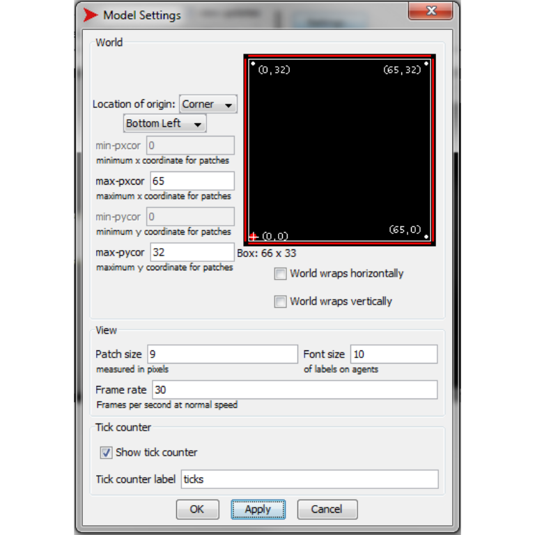
Figure 12.1: Setting the world size and resolution
In addition to the main view of our agents’ world, the other optional views are monitors, plots and an output window.
Monitors report the values of variables. Our model currently has no variables. To demonstrate, add a monitor — either by right-clicking somewhere on the empty interface or by clicking the Add button on the toolbar and selecting Monitor from the dropdown menu next to it. In the dialogue box that appears type count patches in the reporter field and click OK.
Instead of just reporting the current value of a variable, plots report their changing value through time when the model is running, which can be a very useful visual summary of the model’s progress (Figure 12.2). We will set up a plot later on, when we have populated the model with some agents! Finally the output box can be used to output text while the model is running.
12.3.1.2 Controls
The command centre can be used to issue commands on the fly, either to a finished model (even while it is running) or when developing one or testing. We can try it out to begin to design SimpleWorld by typing in the following commands:
observer> ask patches [set pcolor 2]
observer> ask patches [if pxcor < 24 [set pcolor 4]]
observer> ask patches [if pxcor < 12 [set pcolor 6]]
observer> ask patch 6 9 [ set plabel "Zone 1" ]
observer> ask patch 18 9 [ set plabel "Zone 2" ]
observer> ask patch 30 9 [ set plabel "Zone 3" ]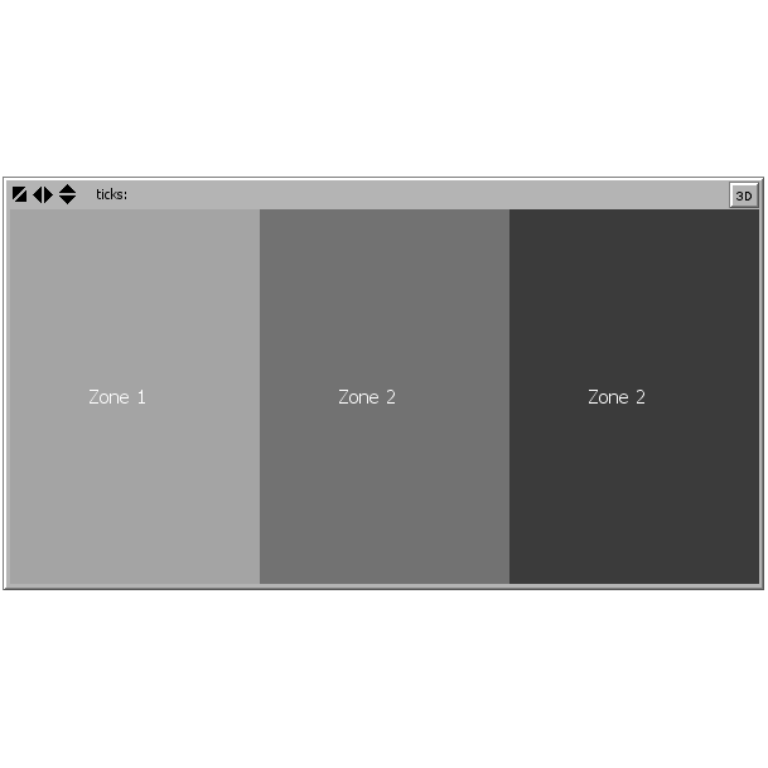
Figure 12.2: SimpleWorld in NetLogo
You will probably find the font size a bit small, in which case you can adjust it in the Graphic Window Settings menu. When we now save, close and reopen our model we will however find that our world — although of the right dimensions — is again black without any zone labels. The Command centre is useful for testing out code snippets like this, but we will have to include these lines in the code tab for them to be saved and run every time.
The second main type of control are the buttons. Although buttons cannot do anything you could not do in the Command centre it is usually convenient to create buttons to call your most used commands and procedures. Most models will therefore have at least a “Setup” button (which is normally run only once at the beginning) and a “Go” button, which continuously executes the commands until it is de-pressed. The commands that are run by the buttons can be simple commands such as the patch colour ones we used above, but more than likely they will be more complex procedures we will define in the code tab. It is good practice therefore to try to keep model procedures in the code tab, so that can be found one place. Alternatively code snippets can go directly inside the button dialogue boxes or run them directly from the Command centre.
Let’s create a button calling the command “setup”. NetLogo will offer a warning “Nothing named setup has been defined.” Now switch to the Code tab and type in the following:
to setup
  clear-all
  create-zones
  reset-ticks
end

to create-zones
  ask patches [set pcolor 2 ]
  ask patches [if pxcor < 24 [set pcolor 4 ]]
  ask patches [if pxcor < 12 [set pcolor 6 ]]
  ask patch 6 9 [ set plabel "Zone 1" ]
  ask patch 18 9 [ set plabel "Zone 2" ]
  ask patch 30 9 [ set plabel "Zone 3" ]
end
The definition of the setup procedure, like all procedures, requires a to opening call and an end to close. All the commands within these two lines will be executed whenever we click on the setup button. The first and last lines are standard in any setup procedure as it will normally be called after a previous model run, so we want to make sure the world is back in starting position and the time or tick counter is set back to zero. The third line calls the create-zones procedure, which is defined underneath. We could have put all the zone-creation commands directly into the setup procedure. But in order to keep the code nicely organized and easier to read, we follow this structure, and separate out logical blocks of code. We can now test the setup button. Note that this procedure is now saved as part of the model.
12.3.1.3 Settings
There are four types of settings widgets: sliders, choosers, switches and input text boxes. These can be used by the user to change specific variables’ values. By adding one of the types of settings widgets we define the global variable that the slider or other type of input modifies, and these variables can then be called in the code. We do not really need to define any selectable inputs at the moment, but let us assume we might want to populate the agents with attributes from different files, and create a chooser that can be used to select the .csv data file. In the dialogue that opens when we add the chooser we define the global variable csv and give it (for now only) a single possible value “agents.csv” (see Figure 12.3).
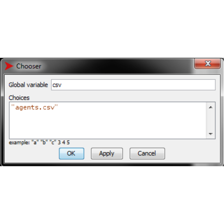
Figure 12.3: SimpleWorld in NetLogo
12.4 Allocating attributes to agents
In order to assign the relevant attributes to the agents we first need to create an appropriately formatted file to be read by NetLogo. The list of 33 agents and their attributes is in the data frame ints_df. In order to read it in NetLogo we first need to export it as a .csv file (making sure the row and column names are not also exported) and place it in the same folder as our .nlogo model:
write.table(ints_df, "NetLogo/agents.csv", row.names=FALSE,
            col.names=FALSE, sep=",")
12.4.1 Defining variables
In NetLogo we can define three types of variables:
- Global variables are at the highest level and are accessible to all agents.
- Agent variables have a unique value for each agent.
- Local variables are defined and accessed only within procedures.
We have already defined the global csv variable when we created the chooser, the other option is to declare a new global variable in the code using globals [ 'variable-name']. Some agent variables are predefined, for example the patches are a type of agent and we have already encountered the variables pcolor and plabel. A user defined patch variable is declared using the command patches-own. Let’s fix the create-zones procedure so that in addition to colouring the patches with correct zones, we also add a zone variable to each patch and give it the correct value:
patches-own [zone]
to create-zones
  ask patches [set pcolor 2 set zone 3]
  ask patches [if pxcor < 24 [set pcolor 4 set zone 2]]
  ask patches [if pxcor < 12 [set pcolor 6 set zone 1]]
  ask patch 6 9 [ set plabel "Zone 1" ]
  ask patch 18 9 [ set plabel "Zone 2" ]
  ask patch 30 9 [ set plabel "Zone 3" ]
end
If we now inspect an individual patch, we will see that it has a new variable zone that holds the correct value for each patch.
Similarly we can define the variables for the agents. The generic agents in NetLogo are called turtles and hence the turtles-own command is used to add agent variables. We can also create our own breed of turtles and call them for example inhabitants. The definition of the new breed has two inputs: the name of the agentset, that is the set off all the agents in the breed and the name for a single agent of that breed. Once we define the breed we can declare its variables as well:42
breed [inhabitants inhabitant]
inhabitants-own [id zone.original age sex income history]
These are the variables from the .csv file. Note that we changed the name of the zone variable because we already have a zone variable that belongs to the patches and, for clarity, because the agents will be able to move around SimpleWorld and it might be useful at some later stage to explore their starting zone. We have also added a variable called history, to record each individual agent’s history for future analysis.
Local variables are defined and accessible only within procedures. For clarity — although this is not necessary — local variable names will commence with %. Reading the code we can then immediately see if a variable is of locally limited scope or if it is a global or agent variable. To keep the code even clearer, we can make sure that we always declare the global, patches-own and other agent variables at the beginning of the code, before we start writing the procedures. Assignments are then made to them using the set command. Local variables are declared on-the-fly (while the model is running) using the let command, and once declared assignments are also made to them using the set command.
12.4.2 Reading agent data - Option 1
Now we need to create a procedure to read the agent data. The read-agent-data procedure needs to:
- open the file, read a single line of data-
- create an
inhabitant - correctly assign the five values to the five inhabitants-own variables
- and place the agent into the correct zone.
We will also assign the agent a colour based on their gender. Then the procedure must repeat this until all the lines of data are read. The first option for accomplishing this is a simple construction, relying on the fact that our current .csv file has a fixed width file format. We know the exact position of each value, because each variable has a constant number of characters.
The NetLogo procedure therefore begins and ends with the file-open and file-close commands, thus opening a connection to the file in question and allowing us to read the data from it. We also use this opportunity to set the default shape of the agents as person. The main loop is a while construction, reading through each individual line and saving it into a local variable (only available within the procedure) %line.43 We then create a single inhabitant and assign the substrings from %line, based on the position of each value, to the appropriate inhabitant’s variables. We also initialize the agent’s history as an empty list: [] and at the end we set the agent’s colour based on their sex and position them on an unoccupied patch in the correct zone.
to read-agent-data
  set-default-shape inhabitants "person"
  file-open csv
  while [not file-at-end?][
     let %line file-read-line
     create-inhabitants 1 [
       set id read-from-string substring %line 0 1
       set zone.original read-from-string substring %line 2 3
       set age read-from-string substring  %line 4 6
       set sex substring %line 8 9
       set income read-from-string substring %line 11 15
       ifelse sex = "m" [set color yellow] [set color green]
       move-to one-of patches with [not any? turtles-here and
         zone = [zone.original] of myself ]
       ]
  ]
  file-close
end
Making sure that we add the read-agent-data procedure to the setup procedure, we can now test our code simply by clicking the setup button on the graphic interface tab. We still have the monitor there counting the patches; let’s edit it to change the reporter instead to something more informative: count inhabitants should do it. Hopefully there are 33 (see Figure 12.4)!
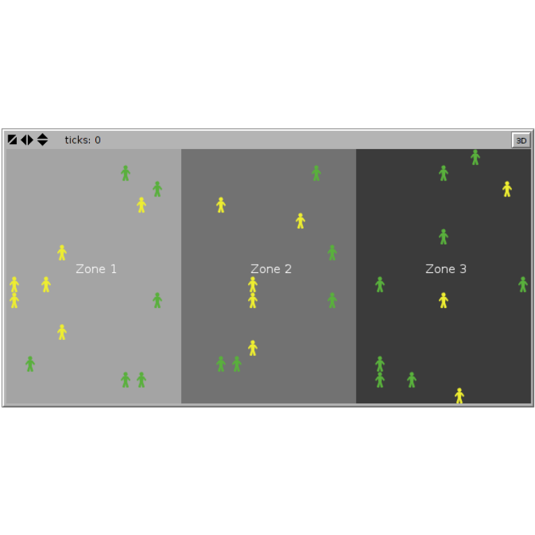
Figure 12.4: SimpleWorld populated with 33 inhabitants
12.4.3 Reading agent data - Option 2
The method of reading in the data described above would not work if SimpleWorld inhabitants had, for example, a five-figure income. A more generic way of reading the data would therefore be to extract the substrings based on the positions of the commas rather than their absolute position. This method is similar to that described above, but it has an extra loop within. Having extracted a single %line, we first add an extra comma to the end of it (using the command word), which will allow us to determine the end position of the last value. The inner loop then finds the position of the first comma and saves it in %pos, reads the value between positions 0 and %pos and saves it as %item, and appends %item to an internal list variable called %data.list. It then removes this item from %line, shortening it by one element, and repeats the loop. This while loop runs until all the items have been extracted individually and saved in %data.list. The rest of the code is similar to the first version: each item is assigned to the inhabitant’s variables, their colour is determined and finally they are positioned in their correct zone.
to read-agent-data-2
  set-default-shape inhabitants "person"
  file-open csv
  while [not file-at-end?][
     let %case file-read-line
     set %case word %case ","
     let %data.list []
     create-inhabitants 1[
       while [not empty? %case] [
         let %pos position "," %case
         let %item read-from-string substring %case 0 %pos
         set %data.list lput %item %data.list
         set %case substring %case (%pos + 1) length %case
         ]
       set id item 0 %data.list
       set zone.original item 1 %data.list
       set age item 2 %data.list
       set sex item 3 %data.list
       set income item 4 %data.list
       ifelse sex = "m" [set color yellow] [set color green]
       move-to one-of patches with [not any? turtles-here and
         zone = [zone.original] of myself ]
     ]
  ]
  file-close
end
To test this option, we simply add read-agent-data-2 to the setup procedure. Make sure you comment out the other read agent procedure - otherwise NetLogo will simply run both of them, populating SimpleWorld with two sets of our 33 inhabitants.
12.5 Running SimpleWorld
We will now create a simple set of rules for the inhabitants of SimpleWorld. At each time tick the inhabitants will:
- move to a random location within their zone.
- “look across the fence”: check their field of vision for inhabitants from a neighbouring zone and select the closest one in view.
- try to “convince” them to come over to the other side: the inhabitant with more money (
income) will bribe the other with 10% of their money to come over to their zone.
The model will have the following adjustable parameters:
- The field of vision has two parameters: the viewing angle and the distance
- Average level of bribeability of inhabitants: if their level is less than 100%, a random number generator will be used to determine whether the agent accepts the bribe or not. The distribution of bribeability is approximately normal with a mean and a standard deviation.
12.5.1 More variable definitions
We first need to define these four global variables using settings widgets. To do this use the add button to add the following four sliders to the model:
| global variable name | minimum | increment | maximum | value | meaning |
|---|---|---|---|---|---|
angle-of-vision |
0 | 10 | 360 | 100 | |
distance-of-vision |
0 | 1 | 10 | 4 | |
average-bribeability |
0 | 1 | 100 | 100 | |
stdev-bribeability |
0 | 1 | 20 | 0 |
The graphic interface area with the aforementioned widget settings should now look approximately like Figure 12.5.
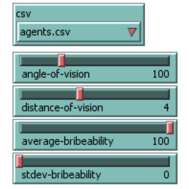
Figure 12.5: New global variables defined using sliders
The average bribeability and its standard deviation that we have just defined will translate into an individual value for each inhabitant. We need to define an agent variable for that purpose. Furthermore, during the bribe negotiations, we need each inhabitant to be in communication with a maximum of one other inhabitant. In order to make sure that happens, we will define a boolean variable to keep track of that. We must therefore add these two variables to the inhabitants-own line (now written over several lines only for clarity):
inhabitants-own [
  id
  zone.original
  age
  sex
  income
  history
  bribeability
  in-negotiations]
12.5.2 More setup procedures
Before we start constructing the Go procedure, we need to add one more setup procedure: one that assigns each agent a random level of bribeability. We will sample from a normal distribution with the mean and standard deviation defined using the sliders. One way of doing that is with the following line:44
ask inhabitants [set bribeability random-normal
  average-bribeability stdev-bribeability ]
The problem with this command, is that the normal distribution is unbounded. But bribeability values below 0% or above 100% make no practical sense. We therefore use the following little trick to force the values into the correct interval:
to determine-bribeability
  ask inhabitants [
    set bribeability median (list 0 (random-normal
      average-bribeability stdev-bribeability) 100) ]
end
Placing the random value in a list with the values 0 and 100 means we can use the median command to extract it when it falls within the interval. But if it falls below 0 the median value of the three will be 0, and similarly if the random normal is over 100, the median will be 100. We can now add the procedure determine-bribeability to the setup procedure, which should be as follows:45
to setup
  clear-all
  create-zones
  ;read-agent-data
  read-agent-data-2
  determine-bribeability
  reset-ticks
end
Try it out with different values for the average and standard deviation of bribeability and make sure it never goes outside the bounds of meaningfulness.
12.5.3 The main Go procedure
We are now ready to write the main action procedure, normally labelled the go procedure. To do that we create a button in the same manner as before, this time running the command go, and make sure we tick the Forever tickbox in the dialogue box. This means clicking the ‘go’ button (with a circular arrow on the face) will execute the command repeatedly, until we stop it manually or until an end condition is met. Let’s first set up the bare bones of the go procedure: in each time step we want the inhabitants to reposition themselves, to engage in the bribery negotiations and we want to record their states in their history variables. Finally we want the tick counter to advance by a single time step:
to go
  ;reposition
  ;engage
  ;record
  tick
end
Because we haven’t defined the first three procedures yet, we are keeping them commented out, as soon as we define them, you should delete the semicolon and test the code.
For repositioning the inhabitants we can use a very similar line of code used to first position the inhabitants in SimpleWorld. To reposition all agents we can use the ask command. NetLogo implements all ask commands sequentially, going through all agents or patches in random order.
to reposition
  ask inhabitants [
    move-to one-of patches with [not any? turtles-here and
      zone = [zone] of myself ]
  ]
end
If we now uncomment reposition in the go procedure, we can test it out. You can adjust the speed of the command execution with the slider on the toolbar at the top of the window.
The construction of the engage procedure is a bit more complex, so let’s break it down into steps:
reset:first we must reset everyone’sin-negotiationsvariable tofalsefind-pairs-and-negotiate:
2.1 find all viable negotiating pairs: ask each inhabitant (not already in negotiations) if there are any viable candidates in their field of vision that are in a different zone. And if so, define these two inhabitants as
partyandcounter-partyrespectively.2.2 then such pairs must
negotiatei.e. compare incomes, determine the winner, transfer the funds and reposition the losing inhabitant into the winner’s zone.
So we therefore need (keeping the unwritten procedures commented out for now):
to engage
  ;reset
  ;find-pairs-and-negotiate
end
The negotiate procedure will be called from find-pairs-and-negotiate and is the last part we will need. For now we will create a place-holder, so we can test the code as we go along. A negotiation will always take place between two inhabitants (labelled the party) and the counter-partyand parties for the turtle-set containing both. It will first of all turn their in-negotiation switch to true, so we know they cannot engage in any other negotiations. We will expand the code to include the actual bribed migration further down. We will only turn their colour red, so we can see who (if anyone) is in negotiations.
to negotiate [ parties ]
  ask parties [
    set in-negotiations  true
    set color red]
end
Next, let’s write the reset procedure, which is very straightforward: at the beginning of each new time step, everyone’s in-negotiation switch is turned back off and everyone’s colour is changed back to what it was before:
to reset
  ask inhabitants [
    set in-negotiations false
    ifelse sex = "m" [set color yellow] [set color green]]
end
The final procedure is find-pairs-and-negotiate which relies on several local variables (prefixed by the % symbol). The pseudo code is as follows:
- for each inhabitant that is not already in negotiations
- define
%field-of-visionas the patches in their sight and also in a neighbouring zone - define
%viable-partnersas all the inhabitants on %field-of-vision, who are available for negotiations
- if there is at least one inhabitant in
%viable-partners, we have a match!
- define the active inhabitant as
%partyand the closest one of the the possible viable partners as%counter-party - now that we have both parties to the negotiations, we can run the
negotiateprocedure on them
The NetLogo code is as follows:
to find-pairs-and-negotiate
  ask inhabitants [
    if in-negotiations = false [
      let %field-of-vision patches in-cone distance-of-vision
        angle-of-vision  with [zone != [zone] of myself]
      let %viable-partners ((inhabitants-on %field-of-vision)
        with [ in-negotiations = false])
      if count %viable-partners > 0 [
          let %party self
          let %counter-party  min-one-of %viable-partners
            [distance myself]
          negotiate (turtle-set %party %counter-party)
          ]
      ]
    ]
end
You should now be able to test the code by uncommenting (by removing the semicolon ; symbol) the engage and go procedures. To actually observe what is happening at each time step, you can edit the go button and untick the Forever option. This way each time you press go, you will get a single repositioning and a single run of engage. You can now already start using two of the sliders: changing the angle and distance of vision of the inhabitants will change the number of inhabitants that engage in negotiations on average. We still have a little count inhabitants monitor in the graphics window, which is not very informative. Edit it instead to change the code to:
count inhabitants with [ in-negotiations = true ]
as well as changing the display name to something shorter. If you’ve done everything right the monitor should only ever show even numbers!
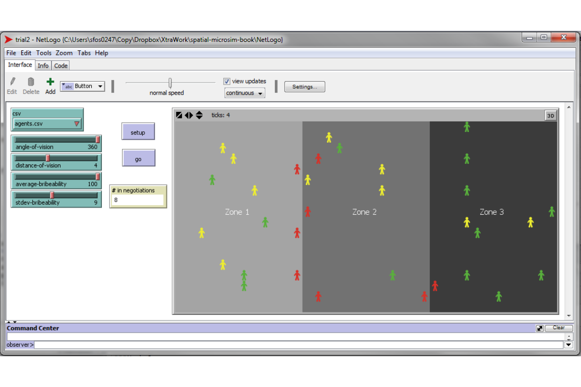
Figure 12.6: SimpleWorld in negotiations
Figure 12.6 is a screenshot of a state of SimpleWorld with 8 inhabitants engaged in active negotiations. Only they are not actually negotiating yet. That is the procedure we left unfinished before and need to rewrite now that we have everything else working. We will break it down into pseudo-code again, in each negotiation we :
- first establish who is the winner and who is the loser using
sort-onon their incomes (if there is a tie,sort-onselects a random winner) - using the loser’s
bribeabilitylevel and a random number generator determine if they will accept the bribe - if so, then transfer 10% of the winner’s income to the loser, and transport the loser into the winner’s zone.
Let’s return to the negotiate procedure we created above as a place-holder and add the actual negotiation to it. We will leave the first three lines from before setting both parties in-negotiations switch to true and colouring them red. The next three lines sort them by income and assign them to either loser or winner. This is followed by an if construct, that only executes if the loser’s bribeability is larger than a random number between 0 and 100. In this case the loser takes the bribe, is moved into the winner’s zone and their colour changes to brown. At the same time the bribe must also be subtracted from the winner’s income.
to negotiate [ parties ]
  ask parties [
    set in-negotiations  true
    set color red]
  let loser-winner sort-on [income] parties
  let loser item 0 loser-winner
  let winner item 1 loser-winner
  if (random-float 100 < [bribeability] of loser)[
    ask loser[
      set income income + 0.1 * [income] of winner
      move-to one-of patches with [not any? turtles-here and
        zone = [zone] of winner]
      set color brown]
    ask winner[
      set income income * 0.9]
    ]
end
We should now have a working model. Go ahead and try it out, e.g. by loading SimpleWorldNetlogo.netlogo.nlogo. After clicking the setup button, you will probably want to adjust the speed in the toolbar to make the model run a bit slower, then simply press Go!
Note that we still have an undefined command record in the go procedure. Depending on what type of analysis we anticipate, we might want to have a full history of what happened in each model run to each of our inhabitants. We can therefore make sure that at every tick the inhabitant’s history variable (a list we initialized in the read-agent-data procedure) gets appended with the agent’s income and zone. We can use the command lput to append the current values to the list:
to record
  ask inhabitants [
     set history lput (list who ticks income zone ) history]
end
Add this procedure to the code and make sure you uncomment record in the go procedure. We will return to the history variable in the final section of this chapter.
12.5.4 Adding plots to the model
After a few repeated model runs the little icons moving around the zones and changing colours will probably become less interesting. You may want another way of visualising what is happening. To do this we can create a couple of plots to summarise what is going on. We will add a line plot that keeps track of the average income in each zone, and another plot displaying the number of inhabitants in each zone. Using the add button from the toolbar we can add a plot somewhere in the empty space in the graphical interface, while making sure there is enough room for both the plots we are planning. A dialogue box will open, where we can first rename the plot to Average Income. Ticking the show legend box is optional. Change the axis ranges to 0 - 500 for the x axis and 2000 - 3000 for the y (don’t worry, as long as you have the Auto-scale box ticked, the plot will automatically adjust when the lines fall out of range). In the pen update commands add the code to plot the mean income of zone 1 inhabitants, which first makes sure there are actually inhabitants in the zone:
if any? inhabitants with [zone = 1] [
plot mean [income] of inhabitants with [zone = 1]]
It is easier to add the code if you click on the pencil icon on the right, where the dialogue box that opens makes it easier to see. Then click on the colour on the left and select a colour and finally change the Pen name to zone 1. Now simply click on the Add pen button and repeat the process for zones 2 and 3, and click OK. You will probably want to increase the size of the plot, by right-clicking it, choosing select and then manipulating the corners of the plot. Now you can re-run the model while the plot updates!
The plotting options in NetLogo are not very extensive. It is possible to create more involved plots using the plotting primitives enabling, for example, an area graph. As before let’s create a new plot and name it Population. Change the axis ranges to 0 - 500 and 0 - 33. Now define the pens as before, but only assign them the correct colour and name. Instead of adding individual pen update commands as before, we will write the plotting commands into the box above, the plot update commands. The reason, as you will see, is that we want the three pens to draw successively, not concurrently (Figure 12.7). We will use the following commands:
set-current-plot-pen "name"specifies which pen we are currently using - the options being the names we gave the pens in the previous stepplot-pen-upandplot-pen-downlift or lower the pen from the plotting area - where pen is by default set downplotxy "value1" "value2"moves the pen to the position determined by the x and y coordinates - depending on whether the pen is down or up, it will either draw or not draw.
In addition we will use a local variable, %total, to keep track of the cumulative total of inhabitants as we go through the three zones, starting from zone 3:
let %total 0
set-current-plot-pen "zone 3"
plot-pen-up
plotxy ticks %total
set %total %total + count inhabitants with [ zone = 3 ]
plot-pen-down
plotxy ticks %total
set-current-plot-pen "zone 2"
plot-pen-up
plotxy ticks %total
set %total %total + count inhabitants with [ zone = 2 ]
plot-pen-down
plotxy ticks %total
set-current-plot-pen "zone 1"
plot-pen-up
plotxy ticks %total
set %total %total + count inhabitants with [ zone = 1 ]
plot-pen-down
plotxy ticks %total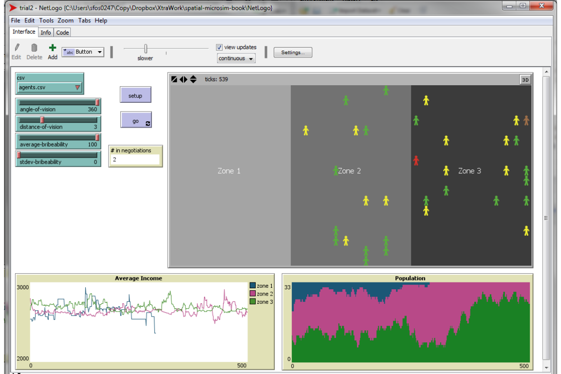
Figure 12.7: Plotting SimpleWorld
12.5.5 Stopping behavior
The last thing to add, to complete the model, is some sort of stopping condition. As it stands the model will keep on running until we de-press the go button. There are several ways of doing this, using the command stop in the go procedure. We could for example insert as the first line into the go procedure the following code: if ticks >= 1000 [ stop ], which will simply stop the model after 1000 iterations. Or we can stop it when a certain criteria is met, such as when all inhabitants end up single zone, using the following code:
if (count inhabitants with [zone = 1] = 33) or
  (count inhabitants with [zone = 2] = 33) or
  (count inhabitants with [zone = 3] = 33) or
  (ticks >= 1000)  [stop]
You will have noticed by now that the model, if left to run, ends up in one of two ways: either with all inhabitants in one zone, or in an indefinite “tie” between zones 1 and 3. Adding the if ticks >= 1000 condition is one way of dealing with the tie issue. But it becomes problematic if we expect the model under some conditions to take longer to reach a single zone winning, so this is not ideal. Another way to avoid the problem of ties is to change the geography of SimpleWorld by wrapping the world horizontally (in the GUI settings menu) which creates a border between zones 1 and 3. SimpleWorld then becomes a vertical cylinder and inhabitants from zones 1 and 3 can bribe each other across their new mutual border.
But in many situations this is not a satisfactory solution and we want to preserve the geography as we originally intended it and allow a tie to be a legitimate end point of the model. So as a final addition to our SimpleWorld ABM we will add some code to keep track of the distribution of inhabitants across the zones and the number of ticks it has remained stable. Then we need to decide on a (rather arbitrary) cut off point after which we declare a tie and stop the model.
To do this we must define two global variables at the beginning of the code. The variable inhabitant-distribution will be a list of three values: the current number of inhabitants in each zone and the variable time-stable will be the number of ticks that have passed since the list has changed.
globals [
  inhabitant-distribution
  time-stable
  ]
We initialize the two variables from the setup procedure, so we add a new procedure start-distribution-tracking at the end of the setup procedure:
to start-distribution-tracking
    set time-stable 0
  set inhabitant-distribution (list
    count inhabitants with [zone = 1]
    count inhabitants with [zone = 2]
    count inhabitants with [zone = 3])
end
Then we have to add a track-distribution procedure that executes at every tick, so we add it to the go procedure - at the end, after record. Each time track-distribution is called we create a local variable new-inhabitant-distribution and compare it to the existing one. If it is the same, we add one tick to the time-stable counter, otherwise we reset the counter back to zero. Finally we replace the old distribution variable with the new one:
to track-distribution
  let new-inhabitant-distribution (list
    count inhabitants with [zone = 1]
    count inhabitants with [zone = 2]
    count inhabitants with [zone = 3])
  ifelse new-inhabitant-distribution = inhabitant-distribution [
    set time-stable time-stable + 1]
  [set time-stable 0]
  set inhabitant-distribution new-inhabitant-distribution
end
We now have a running counter tracking how long it has been since the inhabitant distribution has changed. Now all we need is to decide that e.g. 200 ticks with no change indicates a tie and the simulation can safely be stopped:
if (count inhabitants with [zone = 1] = 33) or
  (count inhabitants with [zone = 2] = 33) or
  (count inhabitants with [zone = 3] = 33) or
  (time-stable >= 100)  [stop]
Now we have a working model to explore. You can try running it with different parameters to see how they affect the behaviour of the model, and you can also try expanding the model to add more. For example a simple way of doing that is by making the 10 % bribe a parameter of the model that can be adjusted by the user. But to systematically investigate the model, we must explore the parameter space by carefully varying all the parameters and recording the results.
NetLogo provides a tool for this called Behaviour Space, which can be found in the Tools menu. It allows you to specify how to vary the variables, how many times to repeat each experiment and which measures to report after each run. Additionally, the tool offers the possibility of running many experiments simultaneously, taking advantage of multi-core processors. Unfortunately this way of doing a parameter sweep is not codeable — the commands defining the experiment are entered in a dialogue box, and the outputs are saved as .csv files, which require further handling for analysis. There are other extensions for NetLogo, such as BehaviourSearch, which can search the parameter space using various search algorithms to optimize an objective function. These and other tools may meet your requirements and/or fit with your workflow. But we will return full circle now back to R and use it to run SimpleWorld and analyse the model results using RNetLogo.
12.6 Control the ABM from R
The RNetLogo package (Thiele 2014) allows us to control a NetLogo model directly from R. Now that we have a working model and have explored it in NetLogo to get a feel for what it’s doing (and make sure that it is doing what we want it to do), we can explore the model more systematically. RNetLogo allows us to issue commands, set global values, repeatedly run the model and collect the results directly from R.
The RNetLogo package is installed in R like any other package using install.packages("RNetLogo"). Note that RNetLogo depends on rJava (Urbanek 2013), which may require some extra configuration of Java, depending on your setup. The basic code for opening and running a model in R is then:
library(RNetLogo)
nldir <- "C:/Program Files (x86)/NetLogo 5.1.0" # program dir
# nldir <- "/home/robin/programs/netlogo-5.1.0/" # e.g. localtion
mdir <- "C:/Users/mz/NetLogo/SimpleWorldVersion2.nlogo" # model dir
# mdir <- "/book_dir/NetLogo/SimpleWorldVersion2.nlogo" # e.g.
NLStart(nldir, gui = FALSE)
NLLoadModel(mdir)

[...main code here ...]

NLQuit()
In the above code NLStart initiates an instance of NetLogo (in this case in headless mode, since the gui argument is set to FALSE — try with gui = TRUE) and NLLoadModel loads the model. Make sure you have the correct paths to the folders where you have installed NetLogo and where the model is saved. Some example directories are commented out for Linux users. The main commands we will want to run in the main code are NLCommand() which simply sends a command for NetLogo to execute, and NLReport(), which also returns a reporter (value). The commands work the same way as if we were entering them in the command center. This also means that the command go is only executed once i.e. not forever as it can be using the GUI button. For example, now that we have opened the model, we can run the following code from R:
NLCommand("setup")
NLReport("ticks")
NLCommand("go")
NLReport("ticks")
The first reporter should have reported the number of ticks to be 0 and the second one should 1, demonstrating that the tick counter has advanced by one. To repeatedly issue a command or report request we can use the NLDoCommand(), so for example:
NLDoCommand(50,"go")
NLReport("ticks")
should now show the tick counter to be 51. We can also repeatedly call a reporter, in this case we have to pass both a command to be repeated a certain number of times and a reporter that will be executed each time. Naturally we can also assign the result to an R variable, and instead of the default list data class return it as a data frame instead:
test <- NLDoReport(10,"go",
                   c(" ticks",
                     "count inhabitants with [zone = 1]",
                     "count inhabitants with [zone = 2]",
                     "count inhabitants with [zone = 3]"),
                   as.data.frame = TRUE)
test # show the resulting data frame

#    X1 X2 X3 X4
# 1  52 11  9 13
# 2  53 11  9 13
# 3  54 11  9 13
# 4  55 11  9 13
# 5  56 12  8 13
# 6  57 12  8 13
# 7  58 12  9 12
# 8  59 12  9 12
# 9  60 12  9 12
# 10 61 12  9 12
Finally we can also extract the current variable values from an agentset. For example the incomes and current zones of all inhabitants, which we can then visualize using a simple boxplot (Figure 12.8):
current.state <- NLGetAgentSet(c("who","income", "zone"),
                               "inhabitants")
boxplot(current.state$income ~ current.state$zone,
  xlab="Zone", ylab="Income",
  main=paste("Income distribution after",
    NLReport("ticks"), "ticks" ))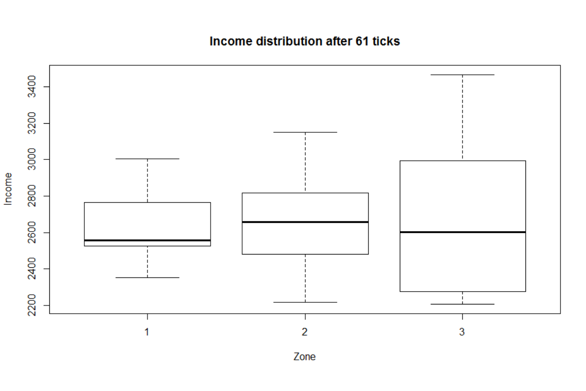
Figure 12.8: NetLogo data plotted in R
The NLCommand and NLReport functions can therefore be executed either singly or repeatedly using their “Do” versions. For ultimate control there are also “Do-While” versions of the functions which take as an argument a condition and keep executing until the condition is met.46
To continue with our simple example the NLDoCommandWhile function could be used simply end the simulation after a certain number of ticks:
NLDoCommandWhile (" (ticks <= 100) " , "go")
NLReport("ticks")
12.6.1 Running a single NetLogo simulation
We now have all the ingredients to run our model from R, and probably do not need to observe the running model in the graphical interface any more. RNetLogo allows us to run the NetLogo silently in the background (in so called headless mode), which runs quite a bit faster than using the GUI. We can also wrap all our NetLogo commands in an R function and make further simulation more modular.
We will set up a single simulation where we open NetLogo silently, load the model, run the simulation until one zone wins or there is a definite tie, and then collect the history of all inhabitants at the end. There is one thing we need to keep in mind running the simulation from R though: we are repeatedly calling a single go procedure. This means we can still continue to call go even if the stopping conditions in the procedure have been met, it simply means the call does nothing. Because there is no warning (or error - nothing went wrong) we have no way of knowing from R that we are continuing to call go which is not doing anything - unless we check the tick counter every time and make sure it has advanced by one.
To run the simulation in R as we had designed it in NetLogo we simply use the same stopping conditions we used in the go procedure. In fact, if you plan to only run your model from R it is a good idea to delete the stopping conditions from the NetLogo code completely and make sure you always define them in the call from R. That way you can avoid setting stopping conditions in R that are less strict than the ones in the model, which would again mean R calling a go procedure that is not doing anything. And be careful: in NetLogo they were stopping conditions, but in NLDoCommandWhile they are exactly the inverse, so make sure you rewrite them appropriately!
SimpleWorld <- function(time.stable = 100) {
  NLCommand("setup")
  NLDoCommandWhile(paste(
    "(count inhabitants with [zone = 1] < 33) and",
    "(count inhabitants with [zone = 2] < 33) and",
    "(count inhabitants with [zone = 3] < 33) and",
    "(time-stable <= ", time.stable, ") ") , "go")
  NLGetAgentSet("history", "inhabitants")
}
The SimpleWorld function can even take an argument that gets passed on to NetLogo: here we have made the number of ticks before we declare a tie adjustable, in case we decide at some point that 100 is not really an appropriate value. Now we can run the simulation and explore the resulting data. Just like R, NetLogo also uses a pseudo random number generator so we can set the random seed we get the same result each time - this may be useful for testing your code and making sure you have set up the simulation the same way as these instructions.
NLQuit() # quit any existing NetLogo instances
NLStart(nldir, gui=FALSE)
NLLoadModel(mdir)
NLCommand("random-seed 42")
inhabitant.histories <- SimpleWorld(50)
We now have the complete history of all 33 inhabitants in the simulation to explore! We can, for example, count how many times each inhabitant moved zones during the simulation and see if that number correlates with their starting income (see Figure 12.9). You can perhaps guess inhabitants with low income will have changed more often, simply because they will have lost more negotiations, but how does the number of moves correlate with their final income? Or with their net income gain during the simulation?
library(dplyr)

history <- as.data.frame(matrix(unlist(inhabitant.histories),
  ncol = 4, byrow = TRUE))
colnames(history) <- c("id", "tick","income", "zone")

changes <- group_by(history, id) %>%
  mutate( change=c(0,diff(zone))) %>%
  summarize(start.income = income[1],
            end.income = tail(income,1),
            income.change = end.income - start.income,
            zone.changes = sum(change != 0))

par(mfrow=c(1,3))
plot(zone.changes ~ start.income , data = changes)
abline(lm(zone.changes ~ start.income , data=changes))
plot(zone.changes ~ end.income , data = changes)
abline(lm(zone.changes ~ end.income , data=changes))
plot(zone.changes ~ income.change , data=changes)
abline(lm(zone.changes ~ income.change , data=changes))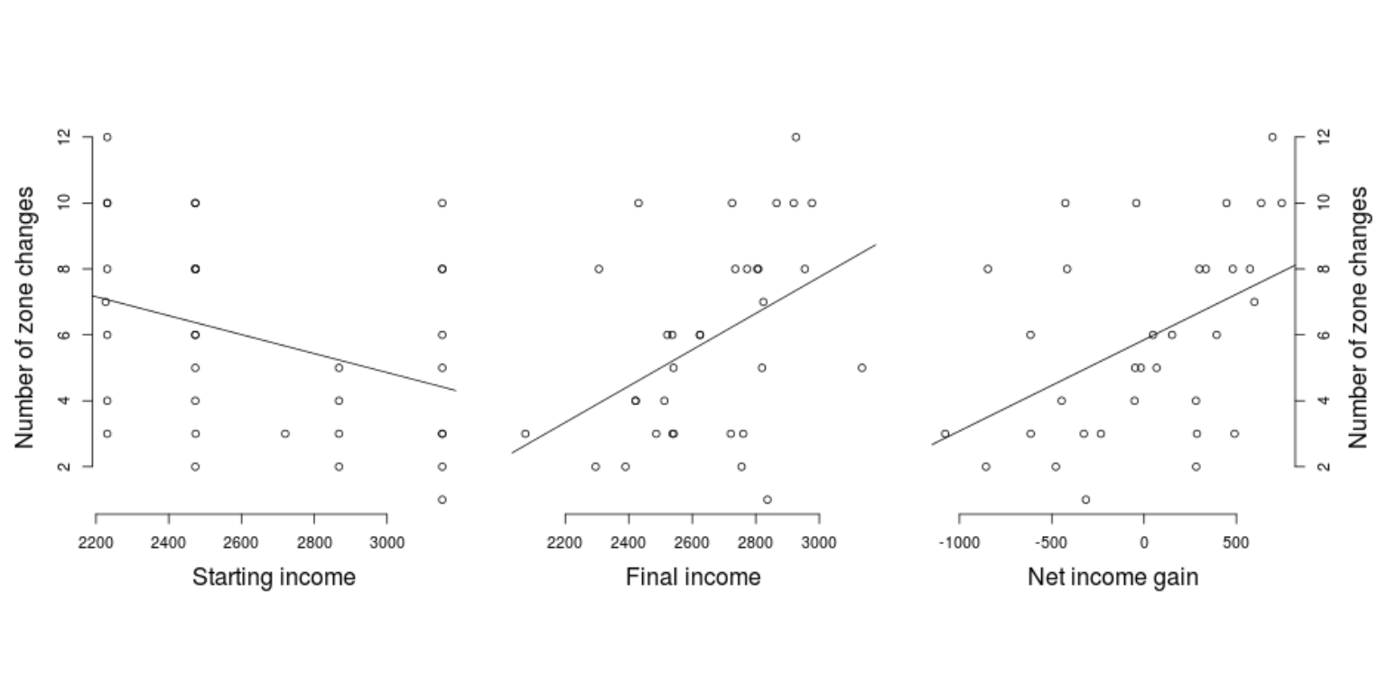
Figure 12.9: Number of zone changes correlated with inhabitants’ income variables
Naturally there are many other things to explore in the history data frame. The flip side of the collected results being so rich is of course that this is a very large data object and its collection during the simulation and importation into R cost valuable resources. The recommended course of action is therefore to explore the history data on a single simulation to decide on what is really of interest. Then change the NetLogo model to only collect the data we are really interested in. In this case we could change the record procedure to only track the number of zone changes for each inhabitant, which would mean simply recovering 33 values at the end of the simulation instead of the full history table, which in this case (a relatively short run) was over 15,000 values. When running multiple simulations exploring the parameter space of the model, as we will do in the next section, collecting such data would be prohibitive.
12.6.2 Running multiple NetLogo simulations
We will focus on a simple outcome variable: the amount of model time (number of ticks) it takes for the simulation to end with clear win for one zone. For simplicity we will treat all simulations that exhibit no changes for over 200 ticks as non-convergent and ignore them. We will explore how this outcome varies depending on the parameters angle-of-vision and distance-of-vision. This is called a full factorial experiment and is only really practical if we have a few parameters to explore, which is why we will stick with only the two variables mentioned.
First let’s rewrite the simulation function to set the appropriate variables before each run (the bribeability variables will not be changing in this simulation, but it is safer to set them explicitly as they may have been changed manually in NetLogo and we would not even notice, because we are running it without the GUI!). After the variables are set, we of course call the setup procedure. We can omit the conditions for running go by simply stopping after nothing has changed for 200 ticks, regardless of how many zones are still in play. After the simulation is finished, we collect two values: the number of ticks minus the value of time-stable, giving us the actual length of the simulation run before it stabilized, and the number of zones that were occupied at the end.47
SimpleWorld <- function(angle.of.vision=360,
  distance.of.vision=10,time.stable = 200) {
  NLCommand (paste("set average-bribeability", 100))
  NLCommand (paste("set stdev-bribeability", 0))
  NLCommand (paste("set angle-of-vision", angle.of.vision))
  NLCommand (paste("set distance-of-vision",
    distance.of.vision))
  NLCommand("setup")
  NLDoCommandWhile(paste("(time-stable <= ", time.stable, ") ")
    , "go")
  c(NLReport(c("ticks - time-stable",
    nrow(unique(NLGetAgentSet( "zone", "inhabitants"))))))
}
The next step is to create a function to run multiple simulations where reps determines the number of repetitions of each parameter value combination and a.o.v and d.o.v determine the value sequences of each parameter that the simulation iterates through. Within it we first create a data frame of the parameter space we intend to examine, with a single row for each simulation run. The function then iterates through this data frame, each time running the SimpleWorld function with the appropriate arguments and collecting these, together with the simulation results, as a data frame with a single row. At the end of all the runs, these are simply binded together into a final data frame with all the results.
MultipleSimulations <-
  function (reps=1, a.o.v = 360, d.o.v = c(5,10)){
  p.s <- expand.grid(rep = seq(1, reps),
    a.o.v = a.o.v, d.o.v = d.o.v)
  result.list <- lapply(as.list(1:nrow(p.s)), function(i)
    setNames(cbind(p.s[i,], SimpleWorld(p.s[i,2], p.s[i,3])),
      c("rep", "a.o.v", "d.o.v", "ticks", "zones")))
  do.call(rbind, result.list)
}
To be on the safe side, we may want to give this function a little test run with only two sets of parameter values and two repetitions each.
results.df <-
  MultipleSimulations(reps = 2, a.o.v = 360, d.o.v = c(5,10))

results.df # display the results data frame

#   rep a.o.v d.o.v ticks zones
# 1   1   360     5    49     2
# 2   2   360     5    94     1
# 3   1   360    10    16     2
# 4   2   360    10    57     1
The first three columns in the results.df data frame are simply the simulation parameters: the number of the repetition and the angle-of-vision and distance-of-vision parameters that were passed to NetLogo. The final two columns give the number of ticks the simulation required to stabilize and the number of zones occupied at the end. Assuming we are happy with the functions, we can now try to running a more serious simulation e.g. five repetitions exploring pretty much the whole of the parameter space - this may take a while!
results.df <- MultipleSimulations(5,seq(60,360,30),seq(1,10) )With the results safely stored in the data frame, we can summarise the data and visualise it.48 Using the dplyr package to reorganize our data we can see how the number of zones occupied at the end of the simulation differed across the parameter space.
zones <- results.df %>%
  group_by(a.o.v, d.o.v, zones) %>%
  summarize(prop.sims = n()/reps) %>%
  group_by(a.o.v, d.o.v)

head(zones) # show the output

# Source: local data frame [6 x 4]
# Groups: a.o.v, d.o.v
#
#   a.o.v d.o.v zones prop.sims
# 1    60     1     3      1.00
# 2    60     2     2      0.15
# 3    60     2     3      0.85
# 4    60     3     1      0.15
# 5    60     3     2      0.75
# 6    60     3     3      0.10
We can see that in the first set of simulations with angle of vision being 60 and the distance of vision only 1, all of the simulations ended with a three-way draw. In the next set, where the distance was set to 2, 85 % of the simulations still ended in a three-way draw, while the remaining 15 % were a two-way draw. Figure 12.10 summarises the data for all 2200 simulations. While there is a clear cluster of three-way ties in the bottom left hand corner, which corresponds to the simulations with the smallest field of vision, there is interestingly no observable pattern to distinguish the two-way ties and single zone simulations.
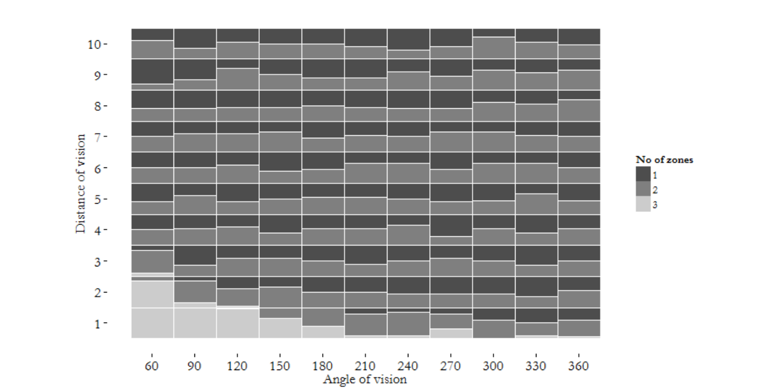
Figure 12.10: Number of zones occupied at end of simulation (20 repetitions)
If we focus on the simulations where a single winning zone emerged, we can find the average number of ticks required across the parameter space:
av.ticks <- results.df %>%
  group_by(a.o.v, d.o.v) %>%
  filter(zones == 1) %>%
  summarize(mean.ticks = mean(ticks, na.rm=TRUE))

head(av.ticks) # display the results

# Source: local data frame [6 x 3]
# Groups: a.o.v
#
#   a.o.v d.o.v mean.ticks
# 1    60     3  1876.6667
# 2    60     4  1577.1000
# 3    60     5   973.6667
# 4    60     6   368.7000
# 5    60     7   265.6000
The average tick counts for all the 2200 simulations (or rather in this case only the 989 that ended with a winning zone) can be plotted as a heatmap (Figure 12.11).
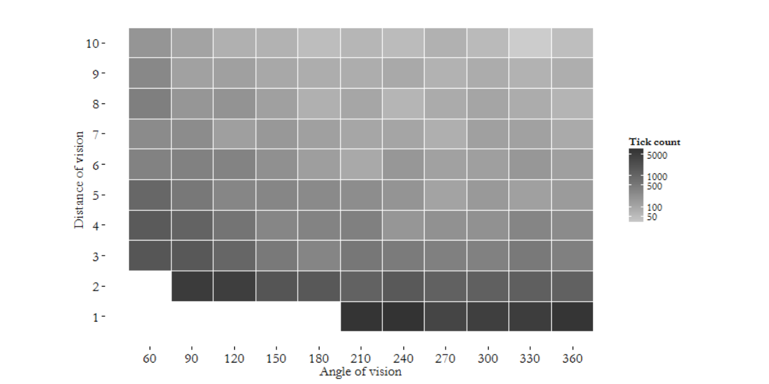
Figure 12.11: Average number of ticks in simulations with single zone winning
12.7 Chapter summary
This is chapter provides a worked example of the numerous options for agent-based modelling building on microsimulation. You have at your disposal a powerful modelling combination when combining NetLogo with R. For an excellent overview with more practical examples see Thiele et al.(2014), which covers a variety of parameter estimation and optimisation methods as well as a comprehensive set of approaches to sensitivity analysis using the RNetLogo setup described here.
References
Lovelace, Robin, and Morgane Dumont. 2016. Spatial Microsimulation with R. CRC Press.
Grimm, Volker, and S F Railsback. 2011. Agent-based and individual-based modeling: a practical introduction. Princeton University Press Princeton, NJ.
Castle, CJE, and AT Crooks. 2006. “Principles and Concepts of Agent-Based Modelling for Developing Geospatial Simulations” 44 (0). doi:ISSN: 1467-1298.
Thiele, Jan C, Winfried Kurth, and Volker Grimm. 2012. “Agent-Based Modelling: Tools for Linking NetLogo And R.” Journal of Artificial Societies and Social Simulation 15 (3): 8. http://jasss.soc.surrey.ac.uk/15/3/8.html.
Thiele, J. 2014. “R Marries NetLogo: Introduction to the RNetLogo Package.” Journal of Statistical 58 (2): 1–41. http://www.jstatsoft.org/v58/i02/paper.
Urbanek, Simon. 2013. rJava: Low-level R to Java interface. http://cran.r-project.org/package=rJava.
Maja is based at the Oxford Institute of Population Ageing, University of Oxford.↩
Although this is not strictly necessary, one recommended structure for your code tab is to break it up into three blocks: 1. Declarations, where you define the global variables, the breeds if any and the agents-own variables; 2. Setup procedures where you define
setupand all its sub-procedures and in a similar vein; 3. Go procedures.↩Using a percentage sign in front of the names of local variables is a purely stylistic decision and makes the code easier to read. It makes it immediately obvious what the scope of each variable is. In NetLogo local variables are created on-the-fly using the
letcommand, while agent and global variables need to be declared explicitly. The values of all variables are changed using thesetcommand.↩You can try it out simply by typing it into the command centre. Seemingly nothing will happen, but if you inspect an inhabitant you will see that their
bribeabilityvariable is now 100.↩Make sure you keep clear-all as the first and reset-ticks as the last procedures.↩
To prevent NetLogo from getting stuck in an endless loop if you inadvertently set a condition that is never met,both of these commands have a
max.minutesargument, the default value of which is 10. The execution will halt after this time has passed before the condition was met. This may be relevant especially if you are expecting to run a long simulation in which case you should increase the value - of course if you are absolutely certain that the condition will be met, then you can also setmax.minutesto 0 and the command will be executed for as long as it takes. In fact for testing your code, when you might be prone to inadvertently writing endless loops, it will make your life easier to change the value to 1 and avoid waiting the 10 minutes it takes for R to stop execution.↩Ensure you remove the history recording from the .nlogo file as it is no longer necessary and will simply slow down the simulations.↩
To smooth out the results the data presented here is based on 20 repetitions.↩