10 Household allocation
So far, this book has explored data on 2 levels: the individual level and the level of administrative zones. The household is another fundamental building block of human organisation around which key decision-making, economic and data-collecting activities are centred. We will here develop results for Belgium in a specific study. Note that this chapter is written by Johan Barthélemy34 and Morgane Dumont. The second part of the chapter is based on a research made by Dumont Morgane (UNamur) and funded by the Wallonia Region of Belgium. Timoteo Carletti (UNamur), Eric Cornélis (UNamur), Philippe Toint (UNamur) and Thierry Eggericks (UCL Louvain-La-Neuve) were involved in the research. The academic groups of DEMO from UCL-Louvain-La-Neuve and the OWS (Observatoire Wallon de la Santé) also provided support.35
This chapter explains how to take spatial microdata, of the type we have generated in the previous chapters, and allocate the resulting individuals into household units.
As with all spatial microsimulation work, the appropriate method for household creation depends on the data available. Data availability scenarios, in descending order of detail, include:
- Access to a sample of households for which you have information about each member.
- Access to separate datasets about individuals and households, stored in independent data tables that are not linked by household ID.
- No access to aggregate data relating to households, but access to some individual level variables related to the household of which they belong (e.g. number of people living with, type of household).
This chapter explains methods for household level data generation in the latter two cases. The first possibility, having a sample of households, is the topic of next chapter (Chapter 11) on the TRESIS method. In this chapter, we focus on the two cases where you have no microdata for the households (meaning data with one row per household).
The chapter is structured as followed:
-Independent data (individuals and households) (10.1) considers the case in which data on households and individuals remain completely separate. -With additional household’s data (10.2.2) presents a strategy when having additional data to the individual data.
Note that the first section explains a method of the literature only theoretically, whereas the second section is developed more in detail and present results for Belgium.
10.1 Independent data (individuals and households)
When the individual level data are independent from the household level data, they can rarely be linked. Data coming from different sources, sometimes implying different total populations, can cause this inconsistency. This section describes the method proposed by Johan Barthélemy for dealing with such situations.
The method is to proceed in three steps. First, we determine the individual distribution Indl, for example by using the package mipfp, as explained before. Second, we determine the distribution of characteristics for the household’s data, hereafter named Hh. This can be done using the same technique as for the individual level data, considering the households instead of the individuals in the previous chapters.
Third, after individual and household level distributions have been estimated, the individuals can be allocated to households. This is done one household at a time by first selecting its type before randomly drawing its constituent members (Barthelemy and Toint 2013).
10.1.1 Household type selection
The household type selection is performed to ensure the distribution of the generated synthetic households is statistically similar to the previously estimated one, i.e. \(Hh\). This is achieved by choosing the type \(hh*\) such that the distribution \(Hh'\) of the already generated households (including the household being built) minimizes the \(\chi^2\) distance between \(Hh'\) and \(Hh\) i.e:
\[d_{\chi^2}=\sum_{i} \frac{(hh'_i-hh_i)^2}{hh_i^2} \]
where \(hh_i\) and \(hh_i'\), respectively, denote the number of households of type \(i\) in the estimated and generated synthetic population. Note that this optimization is simple as the number of household types is limited.
10.1.2 Constituent members selection
Now that a household type has been determined, we can detail the members selection process. First a household head is drawn from the pool of individuals IndPool defined by the estimated individuals distribution Ind. Then, depending on the household types, a partner, children and additional adults are also drawn if necessary. This process is illustrated in Figure 10.1.
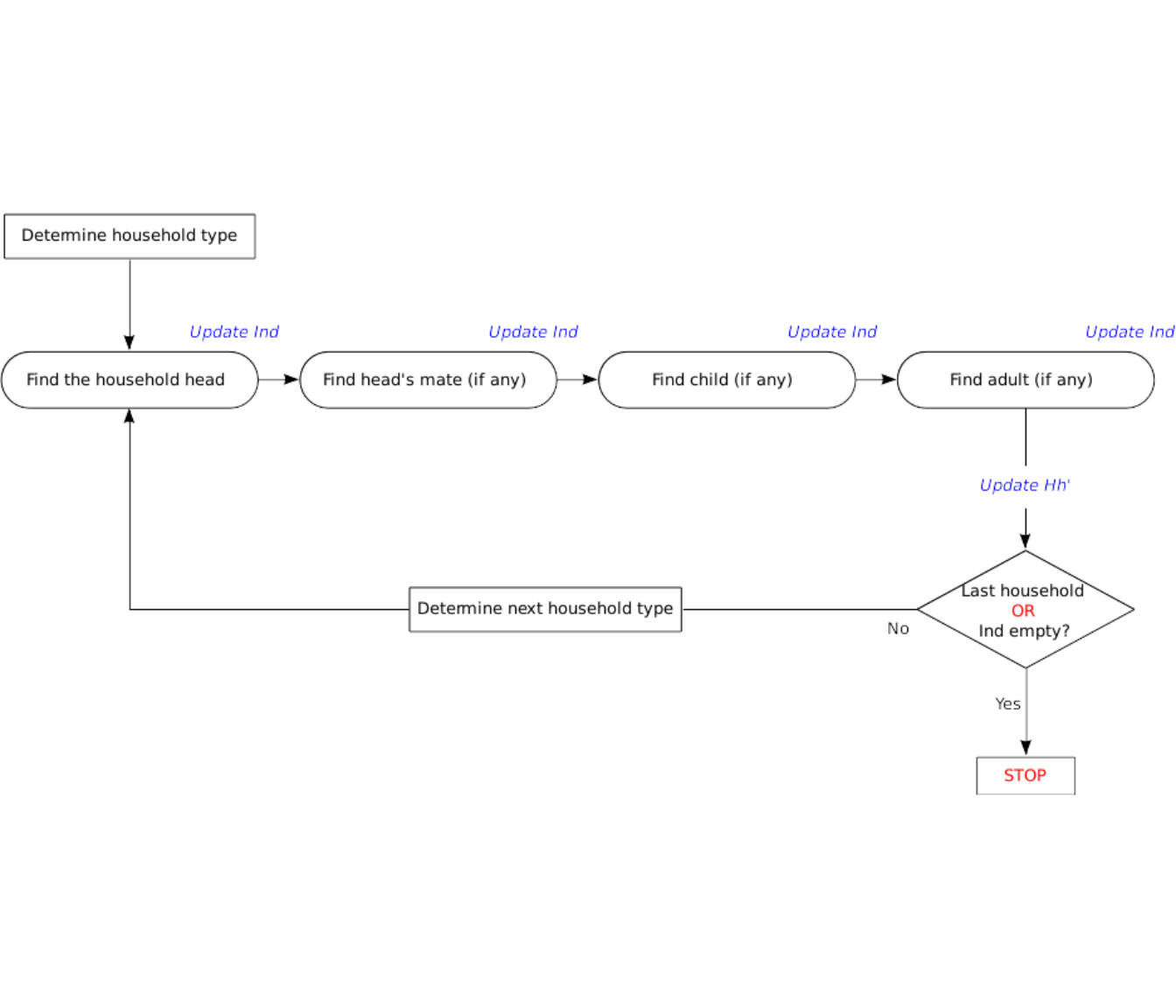
Figure 10.1: Constituent members selection process
Some attributes of the members can be directly obtained from their household type (for instance the gender of the head for an household of the type Isolated Man). The remaining missing attributes are then:
- either randomly drawn according to some known distributions (e.g. the household type x head’s gender x head’s age x mate’s age);
- or, if different values are feasible and equally likely, retained from the distribution which minimizes \(\chi^2\) between generated and estimated distributions. This is similar to what is done for the household type selection.
After an individual type has been determined, then the corresponding member is added to the household being generated:
- if the selected class is still populated in the
IndPool, we extract an individual from this class and add it to the household; - else we find a suitable member by searching in the members of the households already generated. This last individual is then replaced thanks to an appropriate one drawn in
IndPool.
Note if some additional data is available for instance the age difference between partners in a couple, then we can use it to constraint the selection of the current individual type.
10.1.3 End of the household generation process
The household generation process ends after any one of these three conditions: if all households have been constructed; if the pool of individual is empty; or if the process fails to find a member for a household in the previously generated ones. When the procedure stops, two types of inconsistencies may remain in the synthetic population: the final number of households may be smaller than estimated and/or the number of individuals estimated may be less than the known population of the area. In this case, we can form households with the remaining individuals even if they are not probable and then try to make exchanges to improve the fit. These exchanges can be made by following the principles of a tabu search. This consists of an algorithm that remembers the last tries to avoid repeating the same exchange many times (Hongbin Zhang 2002).
10.2 Cross data: individual and household level information
In some cases, information about households is included in the individual dataset. For example, individual level data may include variables on type of household or/and the number of cohabitants in addition to gender and age. This provides cross-tabulated information between the households and the individuals. Considering the microdataset, IPF can help to obtain, per zone, inhabitants described by individual level variables (such as sex, age and income) and some household level information (such as household type and household’s size).
To form the households with this resulting data, we have two possible alternatives. The first is to aggregate the information concerning the individuals and the households independently. By this way, we build two independent tables and we can use an algorithm similar to the one in 10.1. The second possibility aims to preserve the full potential of the data. This means that individuals are joined with the constraints to follow as well as possible their characteristics. For example, two people being head cannot live together; if a person has 3 cohabitants, he needs to be in a household of 4 individuals. The former solution is simpler and requires only the first chapters of the book. However it results in a loss of possible precision. The second possibility, which preserves all the information in individual and household level tables, is explained in this section.
With cross data, we usually proceed in two stages. First, we create the individuals with all their characteristics. The second step is to group these individuals into households using combinatorial optimisation. Each person must be matched to one and only one household.
For this process there are two possible methods. One assumes access to household level variables only in the individual level data. The other assumes access to additional data concerning the structure of the households such as the age difference amongst a married couple. These options are described below.
Note that in both situations, the aim is to form households where each individual is contained in one and only one household. Moreover, each individual must respect, as well as possible, its household’s attributes.
10.2.1 Without additional household’s data
When household level constraints are only contained in the individual’s characteristics, they are often several possible groupings.
Consider the case of our Belgium study where the individual level variables are age, gender, municipality, education level, professional status, size and type of households and link with the household head (e.g. wife, child). A good grouping is one that maximises the number of well-fitted constraints. The perfect grouping would be one in which each individual respects its household size and its type of household, as well as his link with the head. In general, it is impossible to reach a perfect grouping, since the data are not perfect. Indeed, it can happen, for example, that there are an odd number of people who need to live in couple, making it impossible to find a perfect coupling.
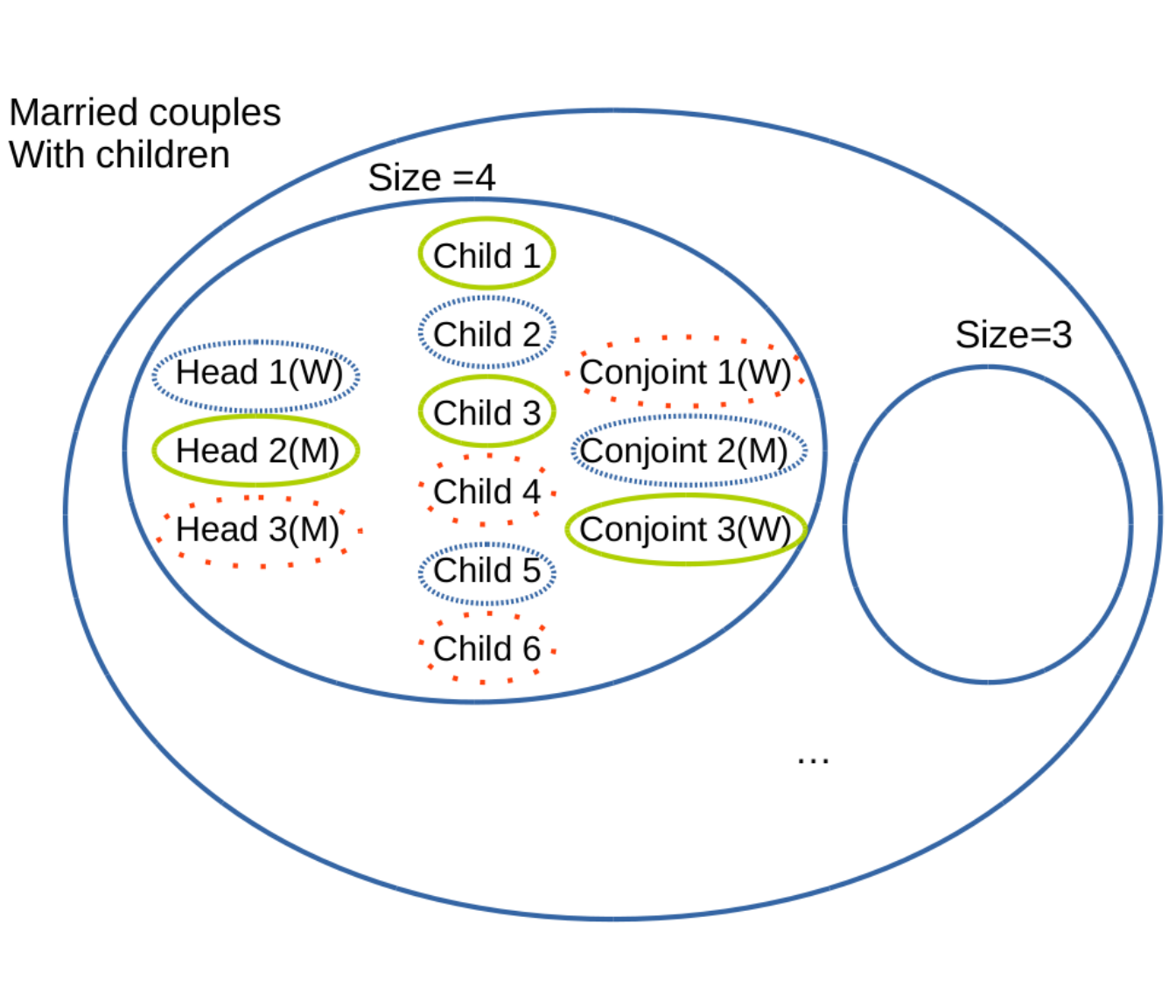
Figure 10.2: Illustration of the problem of grouping members of married couples with children.
As illustrated in Figure 10.2, the individuals can be categorised first by type of household (“married couples with children”" in this case) and then by size of household. This household type has a size of at least 3 (two parents and at least a child). Inside this restricted set of households, the next step is to look at the link that each individual has with the household head and again split the pool of individuals, per link. It is only after this classification that we proceed to the random draw, respecting the links.
For example, for the married couples, we first draw randomly a head and then a partner of the opposite gender (the national register of Belgium for 2011 doesn’t contain homosexual couples). Then, depending on the size of household to be generated, the right number of children are also drawn. This process ends when no additional household can be drawn and respect the constraints. Figure 10.2 shows that we have a household with head 1, who is a woman; partner 2, who is a man; and two children (with ids 2 and 5).
The main sources of error with this method are incoherence in the data and error caused by the IPF process before the grouping. The method implicitly assumes that each household is equally likely to occur, independent of its characteristics.
10.2.2 With additional household’s data
Without additional data on household structure, the only possible method is the one described in 10.2.1. However, this allows improbable households, such as a couple formed by an individual of 18 years old and another of 81 years. For this reason, when we create households, it is often very useful to take into account the differences between age distributions (when these data are available). We can consider the ages within a couple, but also of parents and children.
To do this, we need tables of age differences. These tables are pertinent only when considering variables already included in the simulation (for example, it is impossible to consider a table of age differences per hair color if this variable is not in the model). To explain the process, we develop here the methodology used for the creation of the couples. This means that we have men and women of different ages and roles in the household (head or spouse) and that we need to form the couples. The random draw executed when having no additional data will be improved by considering the real age distributions. Imagine that a part of the additional data is the one in Table 10.1.
| Municipality | Woman’s age | Man’s age | Count |
|---|---|---|---|
| TestCity | 20-25 | 15-20 | 4 |
| TestCity | 20-25 | 20-25 | 25 |
| TestCity | 20-25 | 25-30 | 18 |
| TestCity | 20-25 | 30-35 | 8 |
| TestCity | 20-25 | 35-40 | 2 |
| … | … | … | … |
Note that this is a fictive table, non corresponding to any real data, just to explain the reasoning. Thanks to this table, we know that to fit the real population, we will need 25 couples with a man and a woman, both in the same age class 20-25, etc.
However, these data being not perfect (because coming from different sources with very little variations in the counts or because the synthetic population is not perfect), the marginals could be incoherent with the ones from current synthetic population. For this reason, we will consider the new information only as proportions. For our example, it means that in the total of women having 20-25 years old (57 individuals), \(\frac{4}{57}=0.07=7\)% are married with a man of age 15-20. With this reasoning, we can calculate the new Table 10.2, with a supplementary column considering the proportions.
| Municipality | Woman’s age | Man’s age | Count | Proportion (%) |
|---|---|---|---|---|
| TestCity | 20-25 | 15-20 | 4 | 7 |
| TestCity | 20-25 | 20-25 | 25 | 43.9 |
| TestCity | 20-25 | 25-30 | 18 | 31.6 |
| TestCity | 20-25 | 30-35 | 8 | 14 |
| TestCity | 20-25 | 35-40 | 2 | 3.5 |
| … | … | … | … | … |
These proportions will be useful in next step of the global process. The methodology for the couples with male heads is illustrated in Figure 10.3. For female heads, the process is totally similar.
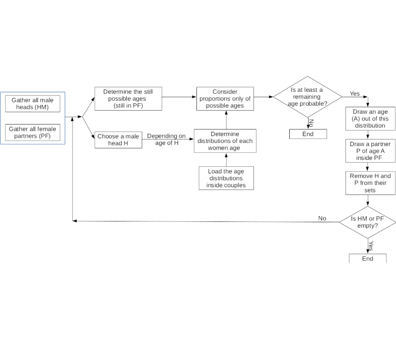
Figure 10.3: Illustration of the algorithm to form the couples
First, we split the set of individuals depending on their role and gender. This forms male heads and female partners to join on one hand, and female heads with male partners on the other hand. We consider each male head turn by turn. For each head, we determine the theoretical distributions of each women ages, depending on the age of the head (thanks to the additional age distribution table). Out of this distribution, we remove the ages that are no more available in the set of possible partners. Indeed, at the end of the process, only a few partners remain to be assigned. Thus, all ages will not be represented any more. Out of this distribution of ages, we calculate the proportions, whose will be used as probabilities in the random draw. Then, thanks to this, we draw an age. Finally, knowing the age of his partner, we choose a wife randomly. This process is repeated until the set of remaining individuals is empty, or there are no remaining partners in the possible ages for the remaining heads.
In our research, this algorithm has been applied to all municipalities in Belgium. The final result is illustrated in Figure 10.4. On this graph, each point corresponds to a combination of (age woman x age man) for a municipality. Its abscissa is the theoretical count for this category, included in the database of the age distributions inside couples. Its ordinate is the number of couples in this category in our synthetic population. Since the dots are on the line formed by the points having both coordinates equal, we can argue that our simulation worked well.
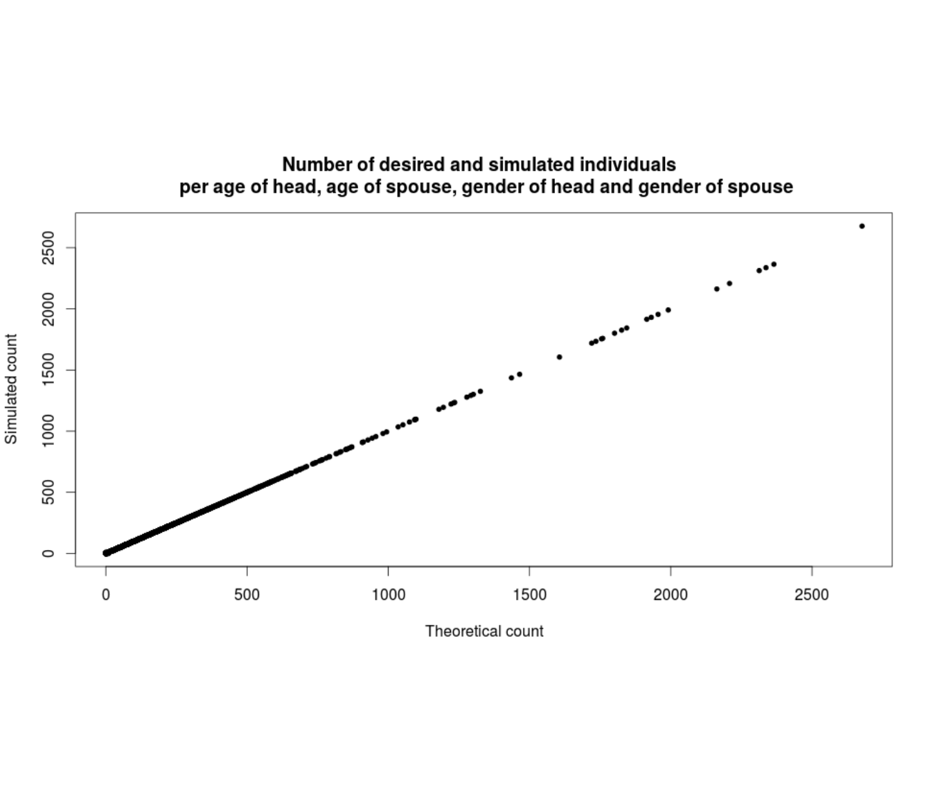
Figure 10.4: Illustration of the results for the couples in Belgium
The assembling of children to the head has been made by a similar process and gives as good results in terms of distribution of ages. However, when no new combination is still possible, some individuals could remain without an assigned household. To improve the spatial microsimulation here, we have chosen to join remaining individuals without regarding at their size of household if this improves the age distribution. This implies less people without an household, but some individuals are in a household not corresponding to its size.
Figure 10.5 indicates that the worst municipality has only 0.5% of non-assigned individuals. The vast majority of the Belgian municipalities has less than 0.1% of these individuals.
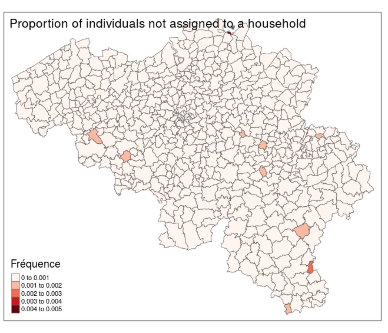
Figure 10.5: Illustration of the non-assigned individuals in Belgium
Figure 10.6 illustrates the proportion of individuals living with a wrong number of cohabitants. In the different municipalities, the proportion varies from 0.7 to 1.05%. These errors affect only a small proportion of each municipality and concern only the size of household (the type of household is always respected).
In conclusion, the simulation fits well the strong contraints (age distributions inside couples and between head and children). The individuals assigned to a household have the right link with the head and most of them live with the right number of cohabitants. Only few individuals has not been chosen to form an household. Thus, we can consider the synthetic population acceptable. Thanks to spatial microsimulation, these new synthetic data are statistically very similar to the real Belgian population. Since these individuals are ‘synthetic’, the resulting population doesn’t suffer of privacy law problems.
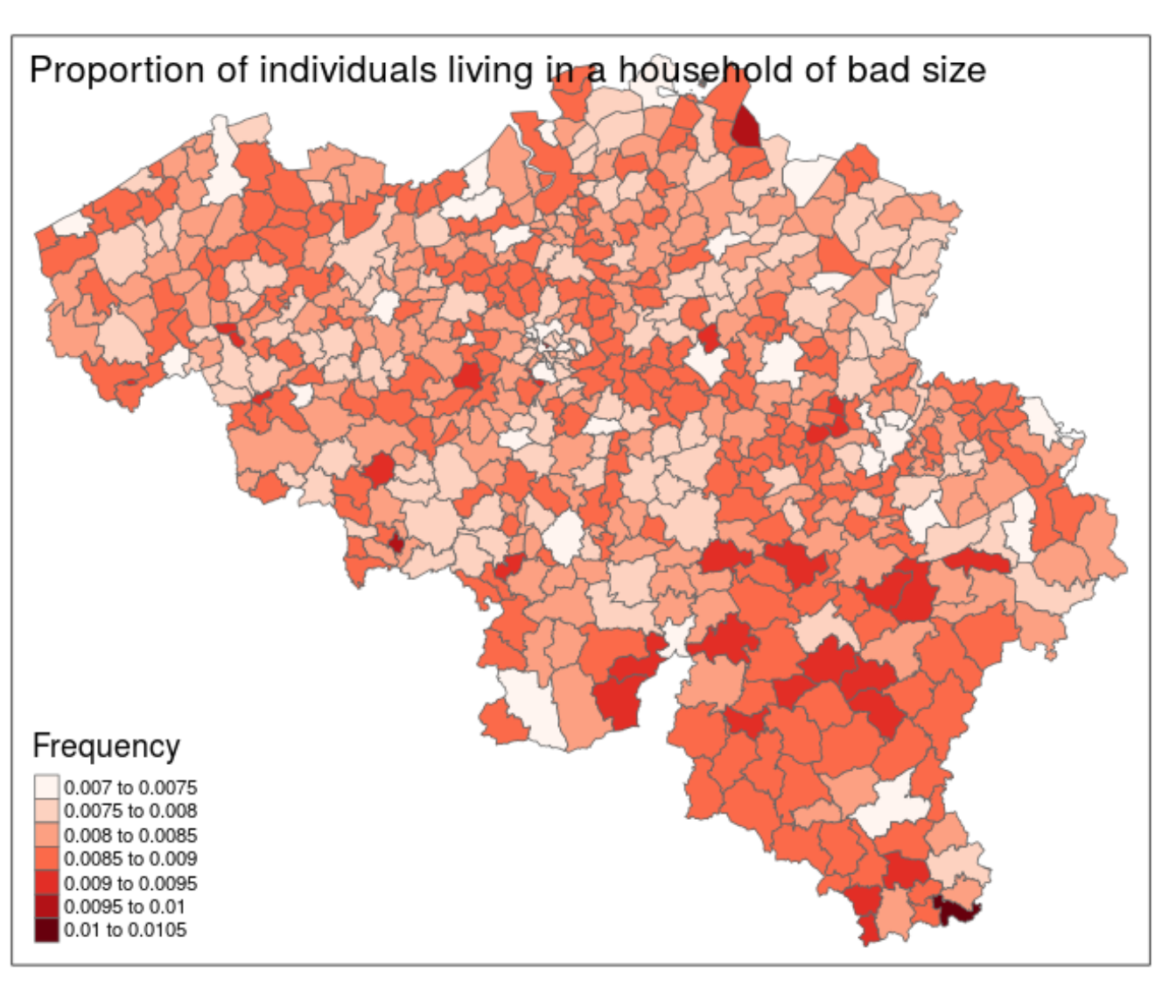
Figure 10.6: Illustration of the individuals in a household of a different size for Belgium
Note that a simulated annealing could be another method to resolve this kind of problems. In our case, we have tested it, but it takes very long CPU time to obtain a result as accurate as the one shown above. However, in cases where the objectives are different, it is possible that a simulated annealing becomes better. Indeed, for our purpose, it worked well, but only the computational time was a major drawback. If you would like to fit age distributions, diploma distributions, and more complicated cases, the simulated annealing could become a good option.
10.3 Chapter summary
This chapter has described methods for allocating individuals into households. Depending on the precision of the available data, the process can result in synthetic households that are more or less representative of the real population. The more pertinent information available, the more realistic will be the resulting households.
References
Barthelemy, Johan, and Philippe L Toint. 2013. “Synthetic Population Generation Without a Sample.” Transportation Science 47 (2). INFORMS: 266–79. doi:10.1287/trsc.1120.0408.
Hongbin Zhang, Guangyu Sun. 2002 35: 701–11.