3 What is spatial microsimulation?

The purpose of this chapter is to demystify the various interpretations and uses of the term ‘spatial microsimulation’ and to define clearly what we mean by it in this book. Following the brief introduction to the field in this first section, the chapter is ordered as follows:

• Terminology (3.1) explains the basis of the concept (3.1.1) and shows how spatial microsimulation can be understood as either a method or an approach (3.1.2).
• What spatial microsimulation is not (3.2) describes the differences between spatial microsimulation and other fields that could seem similar.
• Applications (3.3) explores various academic and real-world applications.
• Assumptions (3.4) addresses the often unspoken assumptions underlying spatial microsimulation results.

For the purposes of this book spatial microsimulation was defined in Chapter 1 as:

The creation, analysis and modelling of individual level data allocated to geographic zones.

Spatial microsimulation is well-suited to the analysis of complex phenomena which happen over geographical space, such as transport systems and housing markets. Because it includes the creation of synthetic data, the method is well-suited to situations in which available data are limited. Figure 3.1 illustrates how the process of population synthesis can be used to impute missing data, by approximating the original geo-referenced individual level data (Lovelace et al. 2015). It is important to note that the process does not stop with the generation of spatial microdata: it involves doing stuff with the spatial microdata to better understand the world.

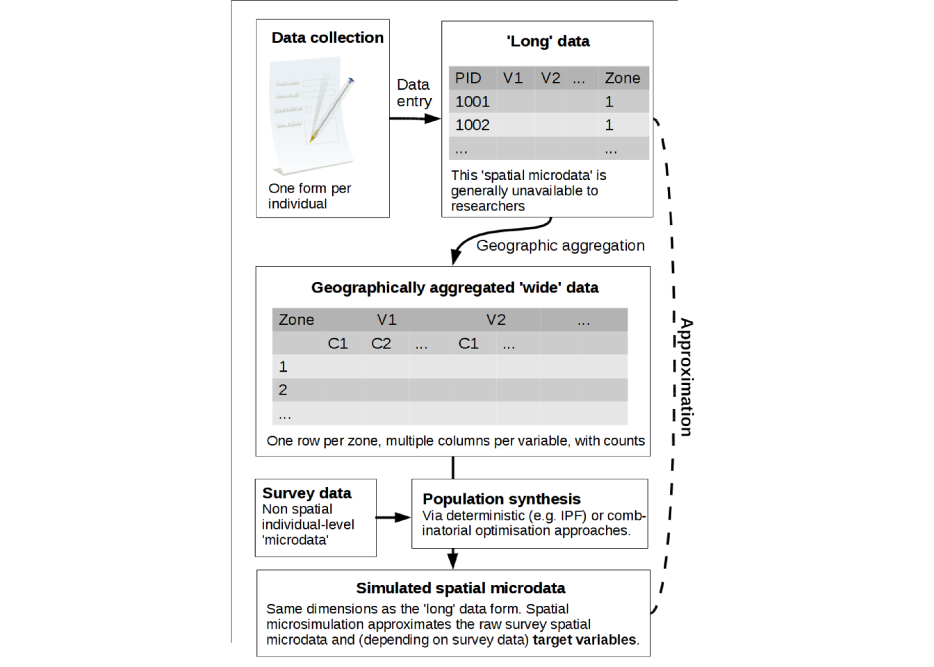
Figure 3.1: Schematic of population synthesis, a critical element in spatial microsimulation

Spatial microsimulation is a way to combine the advantages of individual level data with the geographical specificity of geographical data. If used correctly, it can be used to provide ‘the best of both worlds’ of available data by combining them into a single analysis. Spatial microsimulation should therefore be used in situations where you have access to individual and area level data but no means of combining them. Spatial microsimulation can also be used in contexts where no individual level data is available, as described in Chapter 9.

Typical use cases include modelling the spatial distribution of population growth and changes in demographics; high level transport-modelling; scenario-based modelling of behavioural change; and as an input into agent-based models. Because large individual and area level datasets have only recently become available and because computers have only recently become sufficiently powerful to run large-scale models on thousands of individuals and zones, spatial microsimulation is still a field in its infancy. There are many areas of application where the method has considerable benefits but where the method has not yet been used. It is hoped that this book provides sufficient guidance to enable the reader to use spatial microsimulation on new problems.

3.1 Terminology

Like many phrases, the meaning of spatial microsimulation varies depending on context. The term is more ambiguous than most, however, because it is a relatively new method and because different people have used the term in different ways. Of course, the label attributed to the method is less important than the method itself. As eminent physicist Richard Feynman put it, “the difference between knowing the name of something and knowing something” is vital to understand the world. The methods used in this book could equally be “multi level modelling” or “real-world SimCity”, but this would not change how its methods work or what they do. However, it is important that the terminology we use is at least internally consistent to avoid confusion. Furthermore, it is important to understanding something about how others have used ‘spatial microsimulation’ to avoid misinterpretation of literature that employs the term.

There are some issues with term spatial microsimulation, as described below (see 3.2). However, spatial microsimulation is an appropriate label for the material covered in this book because it is already widely used and because it succinctly conveys the main elements of the approach:

• Spatial microsimulation is inherently concerned with how things vary over space, not just between individuals, groups or periods of time: this is what distinguishes spatial microsimulation from the wider field of microsimulation.
• Spatial microsimulation explores issues at the individual level, as implied by the word micro.
• Spatial microsimulation involves the creation of fictitious data for modelling purposes, captured by the word simulation.

From this breakdown of spatial microsimulation into its component parts its meaning may seem obvious. However, it is important to define the term precisely at an early stage and understand how other people have used the term to avoid confusion.

3.1.1 Spatial microsimulation as SimCity

SimCity is a popular computer game series in which the player constructs urban infrastructure and observes his God-like influence on the virtual citizens. The analogy of SimCity helps to describe spatial microsimulation. In practice, however, the underlying aims of SimCity (entertainment, education and profit for its publisher) are quite different from those of spatial microsimulation research. But, in some ways the comparison is appropriate: SimCity creates virtual individuals allocated to geographic space and provides a framework for model experiments in the same way that spatial microsimulation does. SimCity can be used for teaching urban planning (Gaber 2007) and illustrates how complex computer simulations of urban systems can become. A number of open-source versions of the SimCity concept are now available (e.g. LinCity-NG, Micropolis and Simutrans).

3.1.2 Spatial microsimulation: method or approach?

The most common confusion about what spatial microsimulation is arises because the term has been used to refer to both a narrow methodology and a broader research approach. From Feynman’s distinction between a thing’s label and what it actually is, it is clear that both interpretations are acceptable. The critical step is to use the term in a way that others can understand, remembering that the audience may not have heard of spatial microsimulation before. As stated in the introduction, we acknowledge both uses of the term in the literature but advocate that ‘spatial microsimulation’ is used to describe the overall modelling approach. The term population synthesis, used in transport modelling, is used to describe the methods for generating the spatial microdata on which the spatial microsimulation approach depends.

A subsequent section (3.3) outlines some real-world problems spatial microsimulation has been used to tackle. First, we consider how spatial microsimulation is understood in the literature and how this relates to the definitions used in this book.

Population synthesis is a set of techniques for generating individual level data allocated to geographical zones. Population synthesis is an important (and often crucial) component of the spatial microsimulation approach, the aim of which is to generate a realistic sample for each area that is as similar as possible to aggregate level constraints. Population synthesis usually involves the allocation of individuals from a survey dataset to administrative zones, based on shared variables between the areal (where each unit is a zone) and individual level data. When additional target variables exist in the microdata inputs for population synthesis (which are not present in the aggregate level data), the process can be used to simulate information that is not otherwise available at the local level. Population synthesis in this context can be seen as part of the long-established field of small area estimation (Rao 2003).

Microsimulation (of which spatial microsimulation is a subset) is an approach that was first conceived by Guy Orcutt. This can be defined in general terms as “a methodology … to simulate the states and behaviours of different units — e.g. individuals, households, firms — as they evolve in a given environment” (Baroni and Richiardi 2007). The defining feature of spatial microsimulation is that the ‘environment’ is defined in predominantly geographical terms: the individuals are allocated to small parcels of land which affect their characteristics and inferred behaviour. This wider perspective helps explain why, despite not using the term ‘spatial microsimulation’, Orcutt (1957) is frequently cited as one of the founding fathers of the field.

As with many new and infrequently used words, the term spatial microsimulation is a source of confusion, and its meaning can vary depending on context and who you ask. To an economist, spatial microsimulation is likely to imply modelling a temporal process such as how individual agents in different areas respond to changes in prices or policies. To a transport planner, the term may imply simulating the precise movements of vehicles on the transport network. To your next door neighbour it may mean you have started speaking gobbledygook! Hence the need to consider what spatial microsimulation is, and what it is not, at the outset. However, in every case, the term involves the creation of individual level data that is grouped by geographic zone via some kind of approximation method.

To avoid confusion regarding the terminology used in this book, a glossary defining much of the jargon relating to spatial microsimulation is provided at the end. For now, to help answer what spatial microsimulation is we will look at its applications and then at what it is not.

3.2 What spatial microsimulation is not

Having seen contemporary definitions of spatial microsimulation and what it is, it is also useful to define spatial microsimulation negatively, in terms of what it is not. This is partly due to the close association between spatial microsimulation and other methods, but also because there is a tendency for people to think that spatial microsimulation is more complicated than it is.

Spatial microsimulation is not small area estimation

Small area estimation consists in estimating aggregate counts for a small area. For example, in this field, we can forecast the total population of a zone for a future year. However, we have no information about each individual, it is restricted to statistics on the area. On the other hand, spatial microsimulation really focuses on the micro level. Thus, we estimate the population individual per individual.

Note that, thanks to spatial microsimulation, we are able to aggregate counts and deduce the macro level per municipality, which corresponds to small area estimation.

Spatial microsimulation is not (quite) agent-based modelling

Spatial microsimulation does involve the creation and analysis of individuals and their allocation to families and zone. But it does not necessarily imply interaction between these individuals. For this, agent-based model (ABM) is needed. One could assume that because the method contains the word ‘simulation’, it includes detailed modelling of individual behaviours in which individuals interact with each other and the environment over time and space. This is not always the case: spatial microsimulation is generally a more ‘top down’ approach to modelling, in which the results can be broadly predicted. ABM, by contrast, is bottom-up and can result in highly non-linear and chaotic states (Batty 2005).

There is, however, no clearly defined boundary stating where spatial microsimulation ends and ABM begins and the two approaches are closely linked. The synthetic populations produced as part of spatial microsimulation can form an excellent starting point for ABM. ABM can be seen as an extension of spatial microsimulation. While spatial microsimulation produces individuals and assigns their characteristics over space (and en masse via various ‘what-if’ scenarios), ABMs tend to have higher spatial and temporal resolution, allowing individuals to interact through space and time, with each other and with their environment. This increased level of detail and complexity means that ABM tends to have higher computational needs per individual. As a result, spatial microsimulation models tend to be much larger, encapsulating up to millions of individuals. As computing power continues to increase the potential for adding ABM capabilities to such models is only set to grow (Wegener 2011).

The above discussion illustrates that microsimulation can be seen as a subset of advanced ABM. The results of spatial microsimulation models tend to apply to only specific snapshots in time and individuals tend to be fixed to a single area. ABM can thus add great additional value to spatial microsimulation models, by providing a framework for more complex interactions. Chapter 12 illustrates how the outputs of spatial microsimulation can form an empirical basis for ABM.

In summary, ABM and spatial microsimulation are closely related, overlapping and complementary approaches to the analysis of individual level processes operating over geographical space and time. A main conceptual difference is that the spans of space and time tend to be larger in spatial microsimulation work, for reasons relating to computing power and model complexity.

Spatial microsimulation does not really generate new data

During spatial microsimulation, apparently new individuals are created and placed into zones. It would be tempting to think that new information about the world is somehow being created. This is not the case: the ‘new’ individuals are simply repeats of individuals we already knew about from the individual level data, albeit in a different order and in different combinations. Thus we are not increasing the diversity of the dataset, simply changing its aggregate level characteristics. Spatial microsimulation creates a complete data that take into accounts all other data you included in the process. It is just a way to put all information together to approximate the whole real population, but it does not really generate new data.

Spatial microsimulation is often not strictly spatial

The most surprising feature of spatial microsimulation is that the method is not strictly spatial. The only reason why the method has developed this name (as opposed to ‘small area population synthesis’, for example) is that practitioners tend to use administrative zones, which represent geographical areas, as the grouping variable. However, any mutually exclusive grouping variable, such as age band or number of bedrooms in your house, could be used. Likewise, geographical location can be used as a constraint variable. In most spatial microsimulation models, the spatial variable is a mutually exclusive grouping, interchangeable with any such group. Of course, the spatial microdata, maps and analysis that result from spatial microsimulation are spatial; it’s just that there is nothing inherently spatial about the method used to generate the spatial microdata.

To be more precise, spatial microsimulation is not inherently spatial. Spatial attributes such as the geographic coordinates of the zones to which individuals have been allocated and home and work locations can easily be added to the spatial microdata after they have been generated. It is the use of geographical variables as the grouping variable that is critical here and which distinguishes spatial microsimulation from other types of microsimulation.

A common use of spatial microsimulation (at least the population synthesis aspect) is simply to create model estimates of data which does not exist. This usage case is represented in Figure 3.1, whereby individual level data from a survey is ‘scaled down’ to the local level using population synthesis algorithms. As illustrated in Figure 3.1, the process of population synthesis can be seen as an attempt to reproduce the real spatial microdata collected during the census but which is unavailable for confidentiality reasons.

Input microdata and constraints ensure the simulated results match reality (at least at the aggregate level for the constraint variables — see 3.4). The resulting synthetic spatial microdata is extremely useful for estimating missing data at the local level. If target variables contained in the output were not present in the constraints (income is a common example), estimates of income variability over space can be extracted from the spatial microdata. In addition, the estimated spatial microdata represented in Figure 3.1 will contain estimates of cross-tabulations (contingency tables) between different variables and estimates of the distribution of continuous variables such as age and income. These estimates are useful in many applications (3.3).

3.3 Applications

Spatial microsimulation has a wide variety of applications and there are many areas where the technique has been used. The main areas of application have been health, economic policy evaluation and transport. Rather than attempt to provide a comprehensive account of the range of current and possible applications, this section describes a single study in each area to exemplify how spatial microsimulation is used.

3.3.1 Health applications

A classic example of the potential practical utility of spatial microsimulation is a study which estimated the rate of smoking at the small area level in the city of Leeds UK (Tomintz, Clarke, and Rigby 2008). Smoking is a classic ‘target variable’ in spatial microsimulation: it is reported in a number of individual level surveys but there is surprisingly little information about how smoking rates vary from place to place. Thus it is difficult to determine where to locate services that depend on the rate of smoking. The synthetic spatial microdata could thus be used to help identify new clinics to help people stop smoking. (Alternatively, the spatial microdata could be used by a tobacco chain to help decide where to invest in a new shop, highlighting the potential misuse of the technique by unscrupulous analysts.) The authors found that actual anti-smoking clinics were not located optimally. Furthermore, the results pointed to optimal locations for new clinics, potentially improving the cost-effectiveness of public health campaigns.

This research has since been ‘scaled-up’ to estimate smoking rates across the whole of Austria. The simSALUD portal provides users with access to the resulting spatial microdata and an on-line interface to allow for the selection of constraint variables and other options to customise the model for the specific purposes. This portal-based system and the provision of synthetic spatial microdata to researchers illustrates one possible direction that spatial microsimulation research could go in, where the synthetic data produced from a large model is the main output of the research, to be used by others for a variety of applications.

The example of smoking demonstrates the increase of spatial resolution that spatial microsimulation can bring to bear on under-studied areas in public health. Where the prevalence of unhealthy activities is closely related to socio-demographic variables, a synthetic microdataset can lead to decision making tools that would be difficult to implement with non-spatial surveys alone. Simobesity is another research project and spatial microsimulation software tool that estimates the prevalence of obesity at the local levels depending on demographic constraint variables (Edwards and Clarke 2013). Recent evidence has emerged on the impact of car-dependent urban environments on inactive lifestyles and resulting poor health (these areas have been labelled ‘obesogenic’). In this context, there is great potential for combining socio-demographic and environmental-geographic variables in a spatial microsimulation model. Using the same principles described by Tomintz, Clarke and Rigby (2008), the outputs of such a model could help target local interventions to tackle physical inactivity, maximising the benefits of public health initiatives.

3.3.2 Economic policy evaluation

The social-demographic distribution of impacts arising from economic policy evaluation is one of the most common applications of microsimulation (although the analysis in this area is often non-spatial). ‘Social impact evaluation’, where the impact of policy changes on different income and socio-demographic groups is explored, is a classic example of applied microsimulation research. Frequently these simulations are undertaken by government departments and focus on overall shifts in the population rather than spatial variability in the impacts. The EU–funded EUROMOD project, and software package of the same name, is the largest of these initiatives. The EUROMOD software is used by government analysts and research agencies in many countries to estimate the distributional impacts of policy reforms (Figure 3.2). The resulting research demonstrates that modelling work based on microsimulation can provide important new lines of evidence to inform national level policies (Avram et al. 2012).

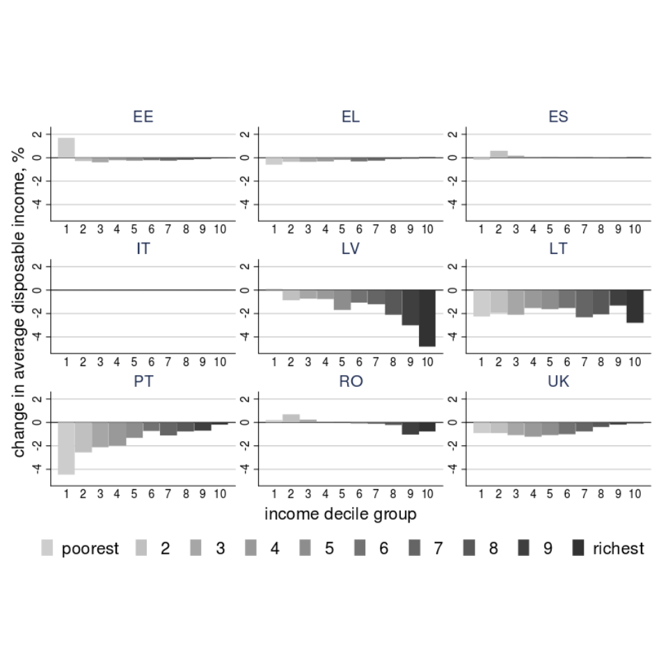
Figure 3.2: Output from the EUROMOD economic microsimulation model (Avram et al. 2014). Along the x axes is income group rising to the right. This means, for example, that Latvia (LV) has implemented progressive policies whereas Portugal (PT) has implemented regressive policies. Country acronyms from left to right stand for Estonia (EE), Greece (EL), Spain (ES), Italy (IT), Latvia (LV), Lithuania (LT), Portugal (PT), Romania (RO) and the UK.

Spatial microsimulation uses very similar techniques as those employed by EUROMOD and other economic microsimulation models, including probability-weighted random sampling of individual level data and aggregate level scenario development (Sutherland and Figari 2013).

The majority of microsimulation research for economic policy evaluation does not disaggregate the impacts over space, however. The estimation of variability at the local level is what differentiates spatial microsimulation models from economic microsimulation models, although the underlying methods are very similar. This book does not cover EUROMOD, focussing instead on spatially disaggregated microdata. However, there is great potential for future work to make EUROMOD more spatially enabled and to bring elements of EUROMOD into the methods outlined in the following chapters.

3.3.3 Transport

Transport modelling is a mature field that increasingly uses individual level data as the basis of analysis. Large scale models such as MATSim rely on spatial microdata to provide demand for travel and individual characteristics for origins and destinations. The same techniques are used in spatial microsimulation and transport modelling generating spatial microdata although in the transport literature, the process is referred to as population synthesis (Axhausen, Müller, and Axhausen 2011).

Generally, little attention is paid to this process of synthetic population generation in transport modelling because the focus is on movement of individuals rather than their characteristics. Distributional impacts are often overlooked in transport models (Lucas 2012) and there is much potential to integrate spatial microsimulation with existing transport modelling methods.

An example of the potential uses of spatial microsimulation in transport models is illustrated in Figure 3.3. This shows the simulated commuting behaviour of 20 randomly selected individuals from a large scale spatial microdataset of Sheffield. Because the constraints used in this model included socio-demographic variables, each individual represented in the figure has a rich profile of characteristics associated with them. This analysis can provide new evidence about the likely winners and losers from very specific interventions such as a new bicycle path or bus route (Lovelace, Ballas, and Watson 2014). As a result of the increased detail allowed by such methods there is much interest in spatial microsimulation for transport applications. Figure 3.3 also illustrates the potential for the output of spatial microsimulation to be used as an input into agent-based models (ABM).

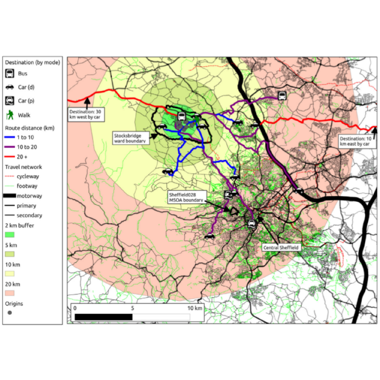
Figure 3.3: An illustration of spatial microdata in transport modelling. 20 people are illustrated on the map as travelling to a range of destinations, specified based on probability-weighted sampling from origin-destination tables (Lovelace et al. 2014).

A larger and more advanced illustration of the potential for spatial microsimulation in transport modelling work is described by Barthelemy and Toint (2015). This paper describes a stochastic model to allocate travel behaviours to a geo-located synthetic population of 10 million people, representing the entirety of the transport system in Belgium. By combining the synthetic microdata with an agent–based modelling approach (described in Chapter 12), Barthelemy and Toint (2015) are able to characterise a very large transport system in great detail.

3.4 Assumptions

As with any simulation technique, spatial microsimulation is based on assumptions, some of which are unlikely to hold in all cases. This does not preclude spatial microsimulation in cases where the assumptions do not hold: “It is far better to foresee even without certainty than not to foresee at all”, as Henri Poincaré put it (Barthélemy 2014).

It is vital, however, that users of spatial microsimulation and ‘consumers’ of the resulting research understand that the results of spatial microsimulation are not real but a best estimate of the population in a given area. The danger is that if the assumptions are not understood, incorrect conclusions will result. It is therefore the duty of researchers using spatial microsimulation (and other techniques) to clearly state the assumptions on which the results depend on and the extent to which these assumptions can be expected to hold in practice. Roughly speaking there are four main assumptions underlying all spatial microsimulation models:

1. The individual level microdata are representative of the study area.
2. The target variable is dependent on the constraint variables and their interactions in a way that is relatively constant over space and time.
3. The relationships between the constraint variables are not spatially dependent.
4. The input microdataset and constraints are sufficiently rich and detailed to reproduce the full diversity of individuals and areas in the study region.

Obviously the real world is complex and many processes are spatially dependent, invalidating assumptions 2 and 3. The extent to which the relationships between variables can be deemed to be constant over space is often unknown. However, there are ways of checking the spatial dependency of relationships between multiply variables, not least Geographically Weighted Regression (GWR).

These limitations should be discussed at the outset of spatial microsimulation research, with reference to the input data. To see how spatial microsimulation simplifies the real world, the next chapter describes a hypothetical scenario where 33 inhabitants of an imaginary land are simulated and allocated to three zones based on a microdataset of only five individuals and two constraint variables.

3.5 Chapter summary

In this chapter we have defined what spatial microsimulation is and what it is not. Some research and real-world applications were described, with comments on areas for further work. The final section on assumptions underlying spatial microsimulation is in some ways the most important: It shows the importance of understanding the limitations associated with the method and the dangers of drawing conclusions from simulated data.

References

Lovelace, Robin, Dimitris Ballas, Mark M.H. Birkin, Eveline van Leeuwen, Dimitris Ballas, Eveline van Leeuwen, and Mark M.H. Birkin. 2015. “Evaluating the performance of Iterative Proportional Fitting for spatial microsimulation: new tests for an established technique.” Journal of Artificial Societies and Social Simulation 18 (2): 21.

Gaber, J. 2007. “Simulating Planning: SimCity as a Pedagogical Tool.” Journal of Planning Education and Research 27 (2): 113–21. doi:10.1177/0739456X07305791.

Rao, Jonathan N K. 2003. Small area estimation. Vol. 331. John Wiley & Sons.

Baroni, Elisa, and Matteo Richiardi. 2007. “Orcutt’s Vision, 50 years on.” October, no. 65. http://ideas.repec.org/p/cca/wplabo/65.html.

Orcutt, Guy H GH. 1957. “A new type of socio-economic system.” The Review of Economics and Statistics 39 (2): 116–23. http://www.jstor.org/stable/10.2307/1928528.

Batty, Michael. 2005. Cities and Complexity. Vol. 14. 1967.

Wegener, M. 2011. “From Macro to Micro—How Much Micro Is Too Much?” Transport Reviews 31 (October 2009): 161–77.

Tomintz, Melanie N M.N., Graham P Clarke, and Janette E J.E. Rigby. 2008. “The geography of smoking in Leeds: estimating individual smoking rates and the implications for the location of stop smoking services.” Area 40 (3). Wiley Online Library: 341–53.

Edwards, KL, and Graham Clarke. 2013. “SimObesity: Combinatorial Optimisation (Deterministic) Model.” Spatial Microsimulation: A Reference Guide for Users, 69–85. doi:10.1007/978-94-007-4623-7.

Avram, Silvia, Francesco Figari, Chrysa Leventi, Horacio Levy, Jekaterina Navicke, Manos Matsaganis, Eva Militaru, Alari Paulus, Olga Rastrigina, and Holly Sutherland. 2012. “The distributional effects of fiscal consolidation in 9 EU countries.” Social Situation Observatory Research Note 01.

Sutherland, Holly, and Francesco Figari. 2013. “EUROMOD: the European Union tax-benefit microsimulation model.” International Journal of Microsimulation 6 (1). Interational Microsimulation Association: 4–26.

Axhausen, KW Kay W, Kirill Müller, and KW Kay W Axhausen. 2011. “Population synthesis for microsimulation: State of the art.” In Annual Meeting of the Transportation Research Board. IVT Working Paper. Swiss Federal Institute of Technology Zurich.

Lucas, Karen. 2012. “Transport and social exclusion: Where are we now?” Transport Policy 20 (March). Elsevier: 105–13. doi:10.1016/j.tranpol.2012.01.013.

Lovelace, Robin, Dimitris Ballas, and Matt Watson. 2014. “A spatial microsimulation approach for the analysis of commuter patterns: from individual to regional levels.” Journal of Transport Geography 34 (0): 282–96. doi:http://dx.doi.org/10.1016/j.jtrangeo.2013.07.008.

Barthelemy, Johan, and Philippe Toint. 2015. “A Stochastic and Flexible Activity Based Model for Large Population. Application to Belgium.” Journal of Artificial Societies and Social Simulation 18 (3): 15. http://jasss.soc.surrey.ac.uk/18/3/15.html.

Barthélemy, Johan. 2014. “A parallelized micro-simulation platform for population and mobility behaviour-Application to Belgium.” PhD thesis, University de Namur.